Testing a Potential Moderator
sze 03 augusztus 2016 by Ernő GólyaThis is part of my coursework for the Data Analysis Tools course by Wesleyan University on Coursera. Week 4 assignment: run an ANOVA, Chi-Square Test or correlation coefficient that includes a moderator.
Moderation is the basic concept of statistical interaction. In statistics, moderation occurs when the relationship between two variables depends on a third variable. The effect of a moderating variable is often characterized statistically as an interaction; that is, a third variable that affects the direction and/or strength of the relation between the explanatory and response variable.
For this post I will test my hypothesis (there is a relationship between child mortality and female education) in the context of a potential
moderating variable (GDP level of the country) by asking the question whether there is an association between the two constructs for different subgroups (income levels) within the sample.
Data source: Gapminder World.
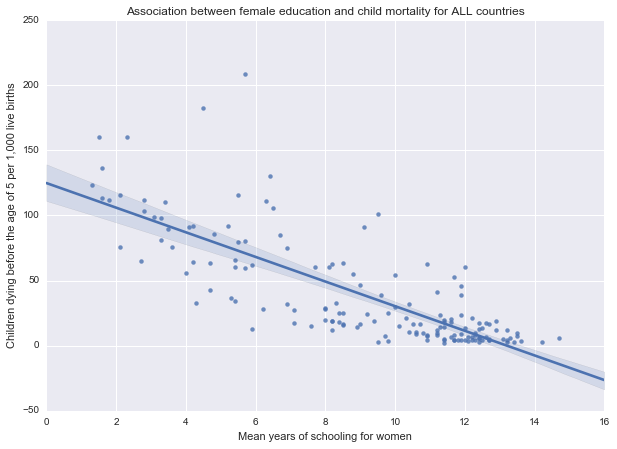
Using Pearson’s correlation coefficient (r), I found that the average time women spend in schools has a significant negative correlation with under-five child mortality rate for the whole data set (r=-0.78, p=1.63e-33). Obviously there may be several potential confounding factors in this association. Now, I want to see if this correlation is dependent on the income level of the country.
The data set contains 154 countries. Incomeperperson is a quantitative variable, so I grouped the observations into 4 income groups (low, lower middle, upper middle, and high) based on the World Bank list of analytical income classification of economies.
incomeperperson_cat:
low: 1-1,005 US$
lower middle: 1,006-3,975 US$
upper middle: 3,976-12,275 US$
high: > 12,275 US$
After running the Pearson correlation test for each group I obtained the following results:
Association between female education and child mortality for ALL countries
(-0.78566944724891918, 1.6315641063941191e-33)
------------------------------------------------------------------------------------------
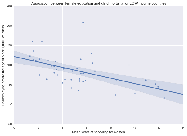
Association between female education and child mortality for LOW income countries
(-0.53543457895633506, 0.000125930575935477)
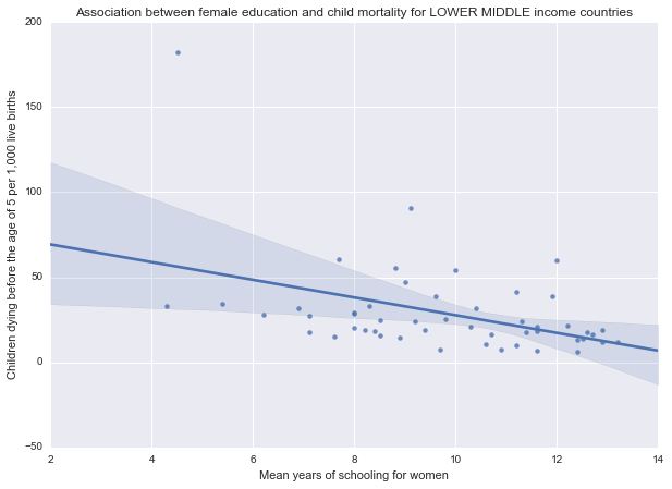
Association between female education and child mortality for LOWER MIDDLE income countries
(-0.42591241118143275, 0.0020437060659682081)
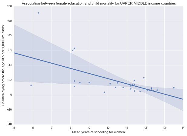
Association between female education and child mortality for UPPER MIDDLE income countries
(-0.60057439538258761, 0.00057180409183018644)
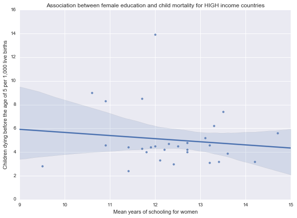
Association between female education and child mortality for HIGH income countries
(-0.12255920495793617, 0.52649555305118811)
As we can see from the results above, there is a statistically significant, moderate negative relationship between female education rates and under-five child mortality rates in low (r=-0.53, p=0.0001; r2=0.28), lower middle (r=-0.42, p=0.002; r2=0.17) and upper middle (r=-0.6, p=0.0005; r2=0.36) income groups. In these countries lower child mortality rates are associated with higher female education rates.
For the high income group, the correlation between female education and under-five child mortality rate is not statistically significant, with a p-value (p=0.52) greater than 0.05. For these countries, we must accept the null hypothesis, that there is no significant relationship between female education and under-five child mortality rate.
(There are 29 countries in the high income category in this data set. In these more affluent countries the average time a woman spend in education is 12.3 years. This may suggest, that above a certain level of educational attainment and income level there is an increased emphasis on other factors affecting child mortality.)
The results are further illustrated by the scatterplots for the different income groups:
Python source code
    # -*- coding: utf-8 -*-
    # Created on 02/08/2016
    # Author Ernő Gólya

    %matplotlib inline
    # import libraries
    import pandas as pd
    import numpy as np
    import scipy.stats
    import seaborn
    import matplotlib.pyplot as plt

    # read in data file
    data = pd.read_csv('custom_gapminder_2.csv', low_memory=False)

    # set variables to numeric
    data["incomeperperson"] = pd.to_numeric(data["incomeperperson"],errors='coerce')
    data["under5mort"] = pd.to_numeric(data["under5mort"],errors='coerce')
    data["womenschool"] = pd.to_numeric(data["womenschool"],errors='coerce')
    data["healthexpend"] = pd.to_numeric(data["healthexpend"],errors='coerce')

    # remove observations with NaN values in any variables of interest
    data = data.dropna()

    # create categories for quantitative variable
    data["incomeperperson_cat"] = pd.cut(data.incomeperperson, [1, 1005, 3975, 12275, 65000],
                                        labels=["Low", "Lower middle", "Upper middle", "High" ])

    # create subgroups of income levels
    subLow = data[(data['incomeperperson_cat'] == "Low")]
    subLowMid = data[(data['incomeperperson_cat'] == "Lower middle")]
    subUpMid = data[(data['incomeperperson_cat'] == "Upper middle")]
    subHigh = data[(data['incomeperperson_cat'] == "High")]

    # generate correlation coefficient for all countries
    print "Association between female education and child mortality for ALL countries"
    print scipy.stats.pearsonr(data['womenschool'], data['under5mort'])
    print "-"*90

    # generate correlation coefficients for income groups
    print "Association between female education and child mortality for LOW income countries"
    print scipy.stats.pearsonr(subLow['womenschool'], subLow['under5mort'])
    print ""

    print "Association between female education and child mortality for LOWER MIDDLE income countries"
    print scipy.stats.pearsonr(subLowMid['womenschool'], subLowMid['under5mort'])
    print ""

    print "Association between female education and child mortality for UPPER MIDDLE income countries"
    print scipy.stats.pearsonr(subUpMid['womenschool'], subUpMid['under5mort'])
    print ""

    print "Association between female education and child mortality for HIGH income countries"
    print scipy.stats.pearsonr(subHigh['womenschool'], subHigh['under5mort'])
    print ""

    # scatterplot for all countries
    fig=plt.figure(figsize=(10, 7), dpi= 80, facecolor='w', edgecolor='k')
    scat1 = seaborn.regplot(x='womenschool', y='under5mort', fit_reg=True, data=data)
    plt.xlabel('Mean years of schooling for women')
    plt.ylabel('Children dying before the age of 5 per 1,000 live births')
    plt.title('Association between female education and child mortality for ALL countries');

    # scatterplot for low income countries
    fig=plt.figure(figsize=(10, 7), dpi= 80, facecolor='w', edgecolor='k')
    scat1 = seaborn.regplot(x='womenschool', y='under5mort', fit_reg=True, data=subLow)
    plt.xlabel('Mean years of schooling for women')
    plt.ylabel('Children dying before the age of 5 per 1,000 live births')
    plt.title('Association between female education and child mortality for LOW income countries');

    # scatterplot for lower middle income countries
    fig=plt.figure(figsize=(10, 7), dpi= 80, facecolor='w', edgecolor='k')
    scat1 = seaborn.regplot(x='womenschool', y='under5mort', fit_reg=True, data=subLowMid)
    plt.xlabel('Mean years of schooling for women')
    plt.ylabel('Children dying before the age of 5 per 1,000 live births')
    plt.title('Association between female education and child mortality for LOWER MIDDLE income countries');

    # scatterplot for upper middle income countries
    fig=plt.figure(figsize=(10, 7), dpi= 80, facecolor='w', edgecolor='k')
    scat1 = seaborn.regplot(x='womenschool', y='under5mort', fit_reg=True, data=subUpMid)
    plt.xlabel('Mean years of schooling for women')
    plt.ylabel('Children dying before the age of 5 per 1,000 live births')
    plt.title('Association between female education and child mortality for UPPER MIDDLE income countries');

    # scatterplot for high income countries
    fig=plt.figure(figsize=(10, 7), dpi= 80, facecolor='w', edgecolor='k')
    scat1 = seaborn.regplot(x='womenschool', y='under5mort', fit_reg=True, data=subHigh)
    plt.xlabel('Mean years of schooling for women')
    plt.ylabel('Children dying before the age of 5 per 1,000 live births')
    plt.title('Association between female education and child mortality for HIGH income countries');