Machine Learning for Data Analysis: K-Means Cluster Analysis

Cluster analysis is an unsupervised machine learning method that partitions the observations in a dataset into a smaller set of clusters where each observation belongs to only one cluster. The goal of clustering is to group observations into a user-specified number (k) of subsets based on their similarity of responses on multiple variables. The correct choice of k is often ambiguous, with interpretations depending on the shape and scale of the distribution of points in a dataset and our desired clustering resolution. Our goal is to obtain clusters that have less variance within clusters and more variance between clusters. In other words, we want observations within clusters to be more similar to each other in their pattern of response on the clustering variables than they are to observations in other clusters. More variance between clusters means the clusters are distinct, there is little or no overlap between them.

One of the most commonly used clustering algorithms is k-means cluster analysis, which is conducted by creating a space that has as many dimensions as the number of input variables. The distance between observations in this space is used to determine how the data points are grouped. The most common way to determine how close observations are to each other is drawing a straight line between pairs of observations, and calculating the distance between them based on the length of the line (Euclidean distance). K-means uses k centroids (points which are the center of a cluster) to define clusters. A point is considered to be in a particular cluster if it is closer to that cluster's centroid than any other centroid. K-means finds the best centroids by alternating between assigning data points to clusters based on the current centroids and chosing centroids based on the current assignment of data points to clusters.

Running a K-Means Cluster Analysis

We run a k-means cluster analysis to identify subgroups of countries based on their similarity of responses on 9 variables that represent characteristics that could have an impact on under-five child mortality. Our goal may be to develop a few targeted interventions to improve child mortality statistics of specific groups of countries based on the characteristics of countries in the clusters. To do this we use a subset of the variables from the gapminder dataset. Basic data management tasks include deleting observations with missing data on any of the variables, creating a dataset that includes only our clustering variables, splitting it into training and test datasets and standardizing clustering variables.

We validate the clusters by excluding under-five mortality rate from the cluster analysis in order to find out if there are differences between the clusters in child mortality. If we do find differences, then we have some evidence that the clusters are valid in terms of identifying subgroups of countries. The specific patterns of child mortality rate related to characteristics on the clustering variables might lead to proposed actions that are more successful in decreasing child mortality rate.

Results of a K-Means Cluster Analysis

A k-means cluster analysis was run to identify underlying subgroups of countries based on their similarity of responses on 9 variables that represent characteristics that could have an impact on under-five child mortality rate. Clustering variables include mean years in school for women, per capita expenditure on health, income per person, estimated HIV prevalence, urban rate, mean age at 1st marriage of women, access to improved sanitation facilities, access to improved drinking water sources and teen fertility rate. All clustering variables were standardized to have a mean of 0 and a standard deviation of 1. Data were randomly split into a training set that included 70% of the observations (N=74) and a test set that included 30% of the observations (N=32). For simplicity, analysis was conducted only on the training dataset.

The Elbow Method

After running a series of k-means cluster analyses on the training data specifying k=1-9 clusters, using Euclidean distance, the variance in the clustering variables that was accounted for by the clusters was plotted for each of the nine cluster solutions in an elbow curve to provide guidance for choosing the optimal number of clusters.

Figure 1. Elbow curve of average distance values for the nine cluster solutions

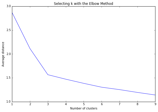
If we plot the average distance explained by the clusters against the number of clusters, the first clusters will add much information, but at some point the marginal gain will drop, giving an angle in the graph. The number of clusters is chosen at this point (elbow). The elbow curve in Figure 1 is quite conclusive, suggesting that the 3-cluster solution might be evaluated. The average distance decreases as the number of clusters increases. Since the goal of cluster analysis is to minimize the distance between observations and the centroids of their assigned clusters we want to choose the fewest number of clusters that provides a low average distance. The bend at 3 clusters shows where the average distance value decreases abruptly, that is, it is leveling off such that adding more clusters doesn't decrease the average distance as much. The results presented below are for an interpretation of this 3-cluster solution.

Canonical Discriminant Analysis

We can plot the clusters in a scatterplot to see whether or not they overlap with each other in terms of their locations in the p dimensional space. However with 9 clustering variables this would mean 9 dimensions. This would be impossible to visualize in a scatterplot, but we use the canonical discriminate analysis, which is a data reduction technique that creates a smaller number of variables that are linear combinations of the clustering variables. Canonical discriminant analysis helps us to reduce the 9 clustering variable down a few variables that accounted for most of the variance in the clustering variables. The scatterplot (Figure 2) shows reasonably clear separation of the 3 clusters for the first two canonical variables. Clusters are distinct and do not overlap with the other clusters, observations in clusters are slightly dispersed suggesting relatively higher variance within clusters. The results of the elbow curve and this plot indicate that the 3-cluster solution is a good solution.

Figure 2. Plot of the first two canonical variables for the clustering variables by cluster.

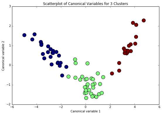
Cluster num., number of observations, color:
0    24    blue
1    32    green
2    18    red

Pattern of Means

Next we can take a look at the pattern of means on the clustering variables for each cluster to see whether they are distinct and meaningful.

Number of countries per clusters
1    32
0    24
2    18

Clustering variable means by cluster
             index  womenschool  healthexpend  incomeperperson     hivrate  
cluster                                                                    
0        79.833333    -1.160504     -0.574122        -0.634139    0.423666   
1        76.562500     0.243558     -0.390768        -0.369349   -0.134883   
2        70.333333     1.095218      1.764662         1.779003   -0.410184   

         urbanrate  ageofmarriage  sanit_pc  watersource_pc  teenfertility  
cluster                                                                     
0        -0.982331      -0.991616 -1.329619       -1.405727       1.127897  
1         0.068667      -0.033505  0.402721        0.456666      -0.191938  
2         1.096177       1.350225  0.937958        0.842825      -0.907623  

The means on the clustering variables show that, compared to the other clusters, countries in cluster 0 (blue) are part of the most disadvantaged areas in terms of the scores of those factors that may have the most significant impact on child mortality. They have the lowest levels of mean years in school for women, per capita expenditure on health, income per person, urban rate, mean age at 1st marriage of women, access to improved sanitation facilities and access to improved drinking water sources. They also have the highest levels of estimated HIV prevalence and teen fertility rate.

Cluster 1 (green) appears to include those countries that have moderate levels on all of the clustering variables.

On the other hand, cluster 2 (red) clearly includes countries with the most favorable indicator data. Countries in cluster 2 have the highest level of mean years in school for women, per capita expenditure on health, income per person, urban rate, mean age at 1st marriage of women, access to improved sanitation facilities and access to improved drinking water sources. They also have the lowest levels of estimated HIV prevalence and teen fertility rate. These countries are likely to have the lowest child mortality rates.

ANOVA - How the clusters differ on under-five mortality

In order to externally validate the clusters, an Analysis of Variance (ANOVA) was conducted to test for significant differences between the clusters on under-five child mortality rate. A tukey test was used for post hoc comparisons between the clusters.

                            OLS Regression Results                            
==============================================================================
Dep. Variable:             under5mort   R-squared:                       0.745
Model:                            OLS   Adj. R-squared:                  0.738
Method:                 Least Squares   F-statistic:                     103.8
Date:                Sun, 04 Sep 2016   Prob (F-statistic):           8.34e-22
Time:                        10:23:45   Log-Likelihood:                -330.43
No. Observations:                  74   AIC:                             666.9
Df Residuals:                      71   BIC:                             673.8
Df Model:                           2                                         
Covariance Type:            nonrobust                                         
===================================================================================
                      coef    std err          t      P>|t|      [95.0% Conf. Int.]
-----------------------------------------------------------------------------------
Intercept          92.8000      4.384     21.167      0.000        84.058   101.542
C(cluster)[T.1]   -67.3437      5.800    -11.612      0.000       -78.908   -55.780
C(cluster)[T.2]   -88.1333      6.697    -13.160      0.000      -101.486   -74.780
==============================================================================
Omnibus:                       18.534   Durbin-Watson:                   1.704
Prob(Omnibus):                  0.000   Jarque-Bera (JB):               26.638
Skew:                           1.016   Prob(JB):                     1.64e-06
Kurtosis:                       5.123   Cond. No.                         3.86
==============================================================================

Warnings:
[1] Standard Errors assume that the covariance matrix of the errors is correctly specified.

Results indicate significant differences between the clusters on child mortality with an F(2, 74)=103.8 and a p<.0001. The tukey post hoc comparisons show significant differences between all clusters on child mortality. Countries in cluster 0 has the highest under-five mortality rate (mean=92.8, sd=31.08), and cluster 2 has the lowest under-five mortality rate (mean=4.66, sd=1.49).

Means for under-five mortality by cluster
         under5mort
cluster            
0         92.800000
1         25.456250
2          4.666667

Standard deviations for under-five mortality by cluster
         under5mort
cluster            
0         31.089436
1         18.389231
2          1.495877



Multiple Comparison of Means - Tukey HSD,FWER=0.05
================================================
group1 group2 meandiff   lower    upper   reject
------------------------------------------------
  0      1    -67.3438  -81.2272 -53.4603  True 
  0      2    -88.1333 -104.1646 -72.1021  True 
  1      2    -20.7896  -35.9377 -5.6414   True 
------------------------------------------------

Python Code

# -*- coding: utf-8 -*-
#
# Created on Sept 03 2016
# @author: Ernő Gólya

%matplotlib inline
import pandas as pd
import numpy as np
import matplotlib.pylab as plt
from sklearn.cross_validation import train_test_split
from sklearn import preprocessing
from sklearn.cluster import KMeans

# data management
data = pd.read_csv("custom_gapminder_3.csv")


variables = ['under5mort','womenschool', 'healthexpend', 'incomeperperson', 'hivrate', 'urbanrate',
                     'ageofmarriage', 'sanit_pc', 'watersource_pc', 'teenfertility',]

# subset with selected variables
data = data[variables]

# convert selected variables to numeric
for variable in variables:
    data[variable] = pd.to_numeric(data[variable],errors='coerce')

# delete observations with missing value(s)
data_nona = data.dropna()

# subset clustering variables
cluster = data_nona.copy().ix[:,1:]

# subset for under5mort ANOVA
u5m_data = data_nona.copy().ix[:,0:1]

# standardize clustering variables to have mean=0 and sd=1
for feature in variables[1:]:
    cluster[feature] = preprocessing.scale(cluster[feature].astype('float64'))

# split dataset into train and test sets
clus_train, clus_test  =   train_test_split(cluster, test_size=0.3, random_state=123)

# k-means cluster analysis for 1-9 clusters
from scipy.spatial.distance import cdist
clusters = range(1, 10)
meandist = []

for k in clusters:
    model = KMeans(n_clusters = k)
    model.fit(clus_train)
    clusassign = model.predict(clus_train)
    meandist.append(sum(np.min(cdist(clus_train, model.cluster_centers_, 'euclidean'), axis = 1)) / clus_train.shape[0])

# Plot average distance from observations from the cluster centroid
# to use the Elbow Method to identify number of clusters to choose
fig=plt.figure(figsize=(9, 6))
plt.plot(clusters, meandist)
plt.xlabel('Number of clusters')
plt.ylabel('Average distance')
plt.title('Selecting k with the Elbow Method');

# interpret 3 cluster solution
model3 = KMeans(n_clusters=3)
model3.fit(clus_train)
clusassign = model3.predict(clus_train)

# plot clusters
from sklearn.decomposition import PCA
pca_2 = PCA(2)
fig=plt.figure(figsize=(9, 6))
plot_columns = pca_2.fit_transform(clus_train)
plt.scatter(x = plot_columns[:,0], y = plot_columns[:,1], c = model3.labels_, s=150)
plt.xlabel('Canonical variable 1')
plt.ylabel('Canonical variable 2')
plt.title('Scatterplot of Canonical Variables for 3 Clusters');

# BEGIN multiple steps to merge cluster assignment with clustering variables
# to examine cluster variable means by cluster

# create a unique identifier variable from the index for the 
# cluster training data to merge with the cluster assignment variable
clus_train.reset_index(level=0, inplace=True)

# create a list that has the new index variable
cluslist = list(clus_train['index'])

# create a list of cluster assignments
labels = list(model3.labels_)

# combine index variable list with cluster assignment list into a dictionary
dclus = dict(zip(cluslist, labels))

# convert dclus dictionary to a dataframe
newclus = pd.DataFrame.from_dict(dclus, orient='index')

# rename the cluster assignment column
newclus.columns = ['cluster']

# now do the same for the cluster assignment variable
# create a unique identifier variable from the index for the 
# cluster assignment dataframe to merge with cluster training data
newclus.reset_index(level=0, inplace=True)

# merge the cluster assignment dataframe with the cluster training
# variable dataframe by the index variable
merged_train = pd.merge(clus_train, newclus, on='index')

# cluster frequencies
merged_train.cluster.value_counts()

# END multiple steps to merge cluster assignment with clustering variables
# to examine cluster variable means by cluster

# calculate clustering variable means by cluster
clustergrp = merged_train.groupby('cluster').mean()
print "Clustering variable means by cluster"
print clustergrp

# validate clusters in training data by examining cluster differences in
# under5mort using ANOVA
# split GPA data into train and test sets
# merge under5mort with clustering variables and cluster assignment data
u5m_train, u5m_test = train_test_split(u5m_data, test_size=0.3, random_state=123)
u5m_train1 = pd.DataFrame(u5m_train)
u5m_train1.reset_index(level=0, inplace=True)
merged_train_all = pd.merge(u5m_train1, merged_train, on='index')
sub1 = merged_train_all[['under5mort', 'cluster']].dropna()

import statsmodels.formula.api as smf
import statsmodels.stats.multicomp as multi

u5mod = smf.ols(formula='under5mort ~ C(cluster)', data=sub1).fit()
print u5mod.summary()

print 'Means for under-five mortality by cluster'
m1 = sub1.groupby('cluster').mean()
print m1
print ""
print ('Standard deviations for under-five mortality by cluster')
m2 = sub1.groupby('cluster').std()
print m2
print "\n\n"
mc1 = multi.MultiComparison(sub1['under5mort'], sub1['cluster'])
res1 = mc1.tukeyhsd()
print res1.summary()