Machine Learning for Data Analysis: Random Forests

The decision tree method introduced briefly in the previous post represents a powerful approach for making predictions based on exploring how many variables can predict a particular target. Decision trees are easy to interpret and visualize and can potentially uncover patterns in our data that can not be easily identified through traditional regression methods. However, even small changes in the data can lead to different results and they are not very reproducible on future data.

Now, let's move on to a related machine learning method, known as Random Forest. This data mining algorithm is a versatile method capable of performing both regression and classification tasks. It can handle a large number of features, and it is helpful for estimating which of our variables are important in the underlying data being modeled.
It belongs to a larger class of machine learning algorithms called ensemble methods which involve the combination of several models to solve a single prediction problem. Random forest aggregates classification (or regression) trees by growing multiple trees (decision tree forest). It works by generating multiple models which make predictions independently, then those predictions are combined into a single prediction. The trees generated are used to collectively rank the importance of variables in predicting our target of interest rather than being interpreted themselves. Thus we get a sense of the most important predictive variables but not necessarily their relationships to one another. To classify a new object based on attributes, each tree gives a classification, the tree “votes” for that class. The forest chooses the classification having the most votes over all the trees in the forest. By trying lots of decision tree variations we can examine which variables are working best or worst in each tree (feature selection). When a certain tree uses one variable and another doesn't, we can compare the effect of the inclusion/exclusion of that variable. Random forest is great for classification. It can be used to make predictions for categories with multiple possible values.

Random forest can be prone to overfitting, especially when working with relatively small datasets, such as the extract from the Gapminder dataset we are going to use to generate a random forest.

Running a Random Forest

Lets take a look at the results of the random forest analysis performed to evaluate the importance of a series of explanatory variables in predicting our binary, categorical response variable (u5_abovemedian, converted from child mortality rate using the global median of the under5mort variable as a cut point). The following explanatory variables were included as possible contributors to the random forest model: mean years in school for women, per capita expenditure on health, income per person, estimated HIV prevalence, urban rate, mean age at 1st marriage of women, corruption perception index, access to improved sanitation facilities, access to improved drinking water sources and teen fertility rate.

Shape of the training and test samples
(63, 10)
(43, 10)
(63,)
(43,)

Much of the code is similar to the code we had written for individual decision trees. The figure above shows the shape of the training and test samples. 63 observations, 60% of the dataset is used as training set. The remaining 40% or 43 observations are used as test set. There are 10 predictors or response variables used in this example. The Random Forest Classifier is initialized with 30 estimators, that is, the random forest is comprised of 30 trees.

Confusion matrix
[[24  0]
 [ 2 17]]

The figure above shows the output of confusion matrix. The diagonal 24, 17 reflects the number of true negatives and true positives respectively. The diagonal 2, 0 reflects the false negatives and false positives for the categorized variable child mortality.

Accuracy score
0.953488372093

The overall accuracy for the forest is 0.95. So 95% of the countries were classified correctly as child mortality rate being above or below the world average.

Relative importance of features

The most helpful information to be obtained from a forest is the measured importance for each explanatory variable (feature), based on how many splits each has produced in the 30 tree ensemble.

Feature ranking:
1. sanit_pc: (0.154530)
2. watersource_pc: (0.151709)
3. incomeperperson: (0.134865)
4. healthexpend: (0.132546)
5. womenschool: (0.127546)
6. ageofmarriage: (0.082550)
7. corrupt_perc: (0.070926)
8. teenfertility: (0.060741)
9. urbanrate: (0.053461)
10. hivrate: (0.031126)

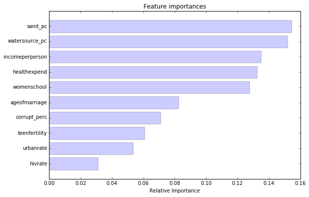
The table and graph show the generated feature importance scores calculated from the forest of trees that we have grown. As we can see the variables with the highest important score are access to improved sanitation facilities (0.15), access to improved drinking water sources (0.15) and income per person (0.13) while the variable with the lowest important score is estimated HIV prevalence at 0.031.

Correct classification rate for different number of trees

To determine what growing larger number of trees brings us in terms of correct classification, we can use code that builds different numbers of trees, and provides the correct classification rate for each. We have used 30 trees in our random forest experiment to achieve this. The figure below shows the accuracy score plotted against the number of trees.

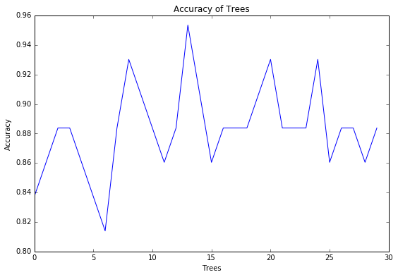
As we can see, with only one tree the accuracy is about 84%, and it climbs up to 95% (at about 12-13 trees), with the subsequent growing of trees adding no more to the overall accuracy of the model.

Python code

# -*- coding: utf-8 -*-
#
# Created on Aug 29 2016
# @author: Ernő Gólya

%matplotlib inline
from pandas import Series, DataFrame
import pandas as pd
import numpy as np
import matplotlib.pylab as plt
from sklearn.cross_validation import train_test_split
from sklearn.tree import DecisionTreeClassifier
from sklearn.metrics import classification_report
import sklearn.metrics
from sklearn import datasets
from sklearn.ensemble import ExtraTreesClassifier

np.random.seed(1234567890)

# data management
inp_data = pd.read_csv("custom_gapminder_3.csv")

variables = ['under5mort', 'womenschool', 'healthexpend', 'incomeperperson', 'hivrate', 'urbanrate',
                     'ageofmarriage', 'corrupt_perc', 'sanit_pc', 'watersource_pc', 'teenfertility']

inp_data1 = inp_data[variables]

data = inp_data1.copy()

# convert selected variables to numeric
for variable in variables:
    data[variable] = pd.to_numeric(data[variable],errors='coerce')

# delete observations with missing value(s)
data2 = data.dropna()

# create u5_abovemedian variable (value = 1 if under5mort > under5median, othervise value = 0)
under5median = data2['under5mort'].median()
def u5_abovemedian(row):
    if row['under5mort'] > under5median:
        return 1
    else:
        return 0

data3 = data2.copy()
data3['u5_abovemedian'] = data3.apply(lambda row: u5_abovemedian(row), axis=1)

print "Median of child mortality rate"
print under5median, "\n"

# create list of predictors
pred_variables = [n for n in variables if n != 'under5mort']

# split dataset into training and testing sets
predictors = data3[pred_variables]
targets = data3.u5_abovemedian
pred_train, pred_test, tar_train, tar_test  =   train_test_split(predictors, targets, test_size=.4)

print "Shape of the training and test samples"
print pred_train.shape
print pred_test.shape
print tar_train.shape
print tar_test.shape

# build model on training set
from sklearn.ensemble import RandomForestClassifier
classifier = RandomForestClassifier(n_estimators = 30)
classifier = classifier.fit(pred_train,tar_train)
predictions = classifier.predict(pred_test)

# print confusion matrix and accuracy score
print "\nConfusion matrix"
cm = sklearn.metrics.confusion_matrix(tar_test, predictions)
print cm
print "\nAccuracy score"
print sklearn.metrics.accuracy_score(tar_test, predictions)
print ""

# fit an Extra Trees model to the data
model = ExtraTreesClassifier()
model.fit(pred_train, tar_train)

# display the relative importance of each attribute
print "Relative importance of features"
print model.feature_importances_
print ""

# Running a different number of trees and see the effect
# of that on the accuracy of the prediction
trees = range(30)
accuracy = np.zeros(30)

for idx in range(len(trees)):
    classifier = RandomForestClassifier(n_estimators = idx + 1)
    classifier = classifier.fit(pred_train, tar_train)
    predictions = classifier.predict(pred_test)
    accuracy[idx] = sklearn.metrics.accuracy_score(tar_test, predictions)

# print the feature ranking
importances = model.feature_importances_
indices = np.argsort(importances)[::-1]
print("Feature ranking:")
for f in range(predictors.shape[1]):
    print "%d. %s: (%f)" % (f + 1, predictors.columns[indices[f]], importances[indices[f]])
indices_rev = np.argsort(importances)
feature_names = predictors.columns[indices_rev]

# plot the feature importances of the forest
plt.figure(figsize=(9, 6))
opacity = 0.2
plt.title("Feature importances")
plt.barh(range(predictors.shape[1]), importances[indices_rev], align="center", alpha=opacity)
plt.yticks(range(predictors.shape[1]), feature_names, rotation='horizontal')
plt.ylim([-1, predictors.shape[1]])
plt.xlabel('Relative Importance')
plt.show()    

print ""

fig=plt.figure(figsize=(9, 6))
plt.plot(trees, accuracy)
plt.xlabel('Trees')
plt.ylabel('Accuracy')
plt.title('Accuracy of Trees');