Regression Modeling in Practice: Multiple Regression Model
v 21 augusztus 2016 by Ernő GólyaThe results of our linear regression model indicated that the level of female education in a country was significantly and negatively associated with the number of children dying under the age of five. But what other variables might explain more of this association and the variability in child mortality?
After we found a significant association in our data, we also want to evaluate whether there are other variables that might confound or explain the relationship. So, the next step is to apply and interpret multiple regression analysis to expand on our research question, and conduct a more rigorous test of the association between under-five mortality and mean years of schooling for women by adding additional variables to our linear regression model. These potential confounding factors are: income per person and per capita total expenditure on health. Our goal is to use regression diagnostic techniques to evaluate how well our multiple regression model predicts the observed response variable (under5mort).
Polynomial Regression Analysis
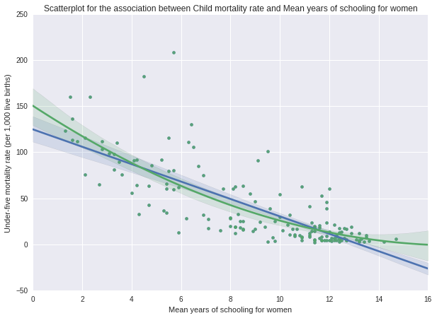
The first order linear scatterplot is an example of a slight curve linear association between female education, and child mortality rate, with a linear regression line. We can fit a line that better fit the association, by adding a polynomial term. We can add a second order polynomial, or quadratic term, to draw the line of best fit that captures the curvature that we're seeing. The scatterplot shows the original linear regression line in blue, and the quadratic regression line in green. It looks like the quadratic curve fits the data better than the straight line, thus quadratic line does a little better job of capturing the association at lower and higher female education levels.
We can be even more sure of this conclusion if we test to see whether adding a second order polynomial term (the squared value of the explanatory variable) to our regression model gives us a significantly better fitting model. First, let's test our regression model for just the linear association between mean years in school for women and under-five mortality rate using the ols function. Note that we have centered our mean years in school for women quantitative explanatory variable.
OLS regression model for the association between schooling of women and child mortality rate
                            OLS Regression Results
==============================================================================
Dep. Variable:             under5mort   R-squared:                       0.617
Model:                            OLS   Adj. R-squared:                  0.615
Method:                 Least Squares   F-statistic:                     245.2
Date:                Sat, 20 Aug 2016   Prob (F-statistic):           1.63e-33
Time:                        09:30:13   Log-Likelihood:                -719.43
No. Observations:                 154   AIC:                             1443.
Df Residuals:                     152   BIC:                             1449.
Df Model:                           1
Covariance Type:            nonrobust
=================================================================================
                    coef    std err          t      P>|t|      [95.0% Conf. Int.]
---------------------------------------------------------------------------------
Intercept        39.7084      2.097     18.932      0.000        35.565    43.852
c_womenschool    -9.4584      0.604    -15.657      0.000       -10.652    -8.265
==============================================================================
Omnibus:                       65.182   Durbin-Watson:                   2.158
Prob(Omnibus):                  0.000   Jarque-Bera (JB):              264.144
Skew:                           1.547   Prob(JB):                     4.38e-58
Kurtosis:                       8.621   Cond. No.                         3.47
==============================================================================

Warnings:
[1] Standard Errors assume that the covariance matrix of the errors is correctly specified.
If we look at the results, we can see from the significant P value (0.000) and negative parameter estimate (Beta=-9.15) that under-five mortality rate is negatively associated with the level of female education. So the linear association, the blue line in the scatter plot, is statistically significant. The R-square is 61.7%, indicating that the linear association of female education is capturing 61.7% of the variability in child mortality rate.
Quadratic OLS regression model for the association between schooling of women and child mortality rate
                            OLS Regression Results
==============================================================================
Dep. Variable:             under5mort   R-squared:                       0.635
Model:                            OLS   Adj. R-squared:                  0.630
Method:                 Least Squares   F-statistic:                     131.3
Date:                Sat, 20 Aug 2016   Prob (F-statistic):           9.07e-34
Time:                        09:31:07   Log-Likelihood:                -715.78
No. Observations:                 154   AIC:                             1438.
Df Residuals:                     151   BIC:                             1447.
Df Model:                           2
Covariance Type:            nonrobust
=========================================================================================
                            coef    std err          t      P>|t|      [95.0% Conf. Int.]
-----------------------------------------------------------------------------------------
Intercept                33.5953      3.055     10.995      0.000        27.558    39.632
c_womenschool            -8.4171      0.706    -11.919      0.000        -9.812    -7.022
I(c_womenschool ** 2)     0.5071      0.188      2.704      0.008         0.137     0.878
==============================================================================
Omnibus:                       82.711   Durbin-Watson:                   2.144
Prob(Omnibus):                  0.000   Jarque-Bera (JB):              434.888
Skew:                           1.933   Prob(JB):                     3.67e-95
Kurtosis:                      10.269   Cond. No.                         26.7
==============================================================================

Warnings:
[1] Standard Errors assume that the covariance matrix of the errors is correctly specified.
But what happens if we allow that straight line to curve by adding a second order polynomial to that regression equation? When we look at the table of results, we see that the value for the linear term for mean years in school is negative (Beta=-8.41), and the p value is less than 0.001. In addition, the quadratic term is positive significant (Beta=0.5, p=0.008), indicating that the curvilinear pattern we observed in our scatter plot is statistically significant. A negative linear coefficient and a positive quadratic coefficient indicates that the curve is convex. In addition, the R square increases to .635, which means that adding the quadratic term for female education, increases the amount of variability in child mortality rate that can be explained by female education from 61.7% to 63.5%. Together, these results suggest that the best fitting line for this association is one that includes some curvature, although the difference is merely 1.8%. 95% Confidence interval: -9.812-(-7.022).
Multiple Linear Regression Model
First we include income per person in the module as a possible confounder in the relationship between the primary explanatory and response variable, then we add total expenditure on health. If we take a look at the parameter estimate for mean years in school after adding a second independent variable income per person, we see that it is -7.21, with p<0.001. If we look at the confidence interval we see that it ranges from -8.89 to -5.2, meaning that we're 95% certain, that the true population parameter for the association between female education, and child mortality falls somewhere between -8.89 to -5.2. R-square is 64.4%. Also note that income per person variable have a Beta=-0.0006 with a p value of 0.016 which is statistically significant. 95% Confidence interval is really small: -0.001-(-0.000). We can reject the null hypothesis of no association between female education and under-five mortality, after adjusted for income per person in the model.
                         OLS Regression Results
==============================================================================
Dep. Variable:             under5mort   R-squared:                       0.649
Model:                            OLS   Adj. R-squared:                  0.642
Method:                 Least Squares   F-statistic:                     92.40
Date:                Sat, 20 Aug 2016   Prob (F-statistic):           6.45e-34
Time:                        10:15:04   Log-Likelihood:                -712.79
No. Observations:                 154   AIC:                             1434.
Df Residuals:                     150   BIC:                             1446.
Df Model:                           3
Covariance Type:            nonrobust
=========================================================================================
                            coef    std err          t      P>|t|      [95.0% Conf. Int.]
-----------------------------------------------------------------------------------------
Intercept                31.8698      3.089     10.318      0.000        25.767    37.973
c_womenschool            -7.2135      0.852     -8.463      0.000        -8.898    -5.529
I(c_womenschool ** 2)     0.6502      0.194      3.358      0.001         0.268     1.033
c_incomeperperson        -0.0006      0.000     -2.439      0.016        -0.001    -0.000
==============================================================================
Omnibus:                       87.976   Durbin-Watson:                   2.129
Prob(Omnibus):                  0.000   Jarque-Bera (JB):              518.390
Skew:                           2.035   Prob(JB):                    2.71e-113
Kurtosis:                      11.014   Cond. No.                     1.60e+04
==============================================================================

Warnings:
[1] Standard Errors assume that the covariance matrix of the errors is correctly specified.
[2] The condition number is large, 1.6e+04. This might indicate that there are
strong multicollinearity or other numerical problems.

                            OLS Regression Results
==============================================================================
Dep. Variable:             under5mort   R-squared:                       0.644
Model:                            OLS   Adj. R-squared:                  0.637
Method:                 Least Squares   F-statistic:                     90.31
Date:                Sat, 20 Aug 2016   Prob (F-statistic):           1.94e-33
Time:                        09:31:38   Log-Likelihood:                -713.93
No. Observations:                 154   AIC:                             1436.
Df Residuals:                     150   BIC:                             1448.
Df Model:                           3
Covariance Type:            nonrobust
=========================================================================================
                            coef    std err          t      P>|t|      [95.0% Conf. Int.]
-----------------------------------------------------------------------------------------
Intercept                31.9783      3.144     10.170      0.000        25.765    38.191
c_womenschool            -7.4624      0.860     -8.681      0.000        -9.161    -5.764
I(c_womenschool ** 2)     0.6412      0.199      3.227      0.002         0.249     1.034
c_healthexpend           -0.0027      0.001     -1.914      0.058        -0.005  8.76e-05
==============================================================================
Omnibus:                       86.986   Durbin-Watson:                   2.139
Prob(Omnibus):                  0.000   Jarque-Bera (JB):              499.466
Skew:                           2.018   Prob(JB):                    3.49e-109
Kurtosis:                      10.846   Cond. No.                     2.77e+03
==============================================================================

Warnings:
[1] Standard Errors assume that the covariance matrix of the errors is correctly specified.
[2] The condition number is large, 2.77e+03. This might indicate that there are
strong multicollinearity or other numerical problems.

                            OLS Regression Results
==============================================================================
Dep. Variable:             under5mort   R-squared:                       0.649
Model:                            OLS   Adj. R-squared:                  0.640
Method:                 Least Squares   F-statistic:                     69.01
Date:                Sat, 20 Aug 2016   Prob (F-statistic):           5.98e-33
Time:                        09:32:02   Log-Likelihood:                -712.66
No. Observations:                 154   AIC:                             1435.
Df Residuals:                     149   BIC:                             1451.
Df Model:                           4
Covariance Type:            nonrobust
=========================================================================================
                            coef    std err          t      P>|t|      [95.0% Conf. Int.]
-----------------------------------------------------------------------------------------
Intercept                32.0983      3.130     10.255      0.000        25.913    38.283
c_womenschool            -7.2760      0.864     -8.425      0.000        -8.982    -5.569
I(c_womenschool ** 2)     0.6313      0.198      3.191      0.002         0.240     1.022
c_incomeperperson        -0.0008      0.001     -1.571      0.118        -0.002     0.000
c_healthexpend            0.0015      0.003      0.499      0.619        -0.004     0.007
==============================================================================
Omnibus:                       87.565   Durbin-Watson:                   2.126
Prob(Omnibus):                  0.000   Jarque-Bera (JB):              513.463
Skew:                           2.025   Prob(JB):                    3.18e-112
Kurtosis:                      10.976   Cond. No.                     1.64e+04
==============================================================================

Warnings:
[1] Standard Errors assume that the covariance matrix of the errors is correctly specified.
[2] The condition number is large, 1.64e+04. This might indicate that there are
strong multicollinearity or other numerical problems.
If we add per capita total expenditure on health to the model, mean years in school for women still has a negative, significant association with child mortality (Beta=-7.27, p<0.001, R2=64.9%). We can still reject the null hypothesis of no association between female education and under-five mortality, after adjusted for both income per person and expenditure on health in the model. Income per person has no longer significant relationship with child mortality (p=0.118) and the same applies to health expenditure, which has a p value of 0.619. In this model, the secondary independent variables are not confounders for the relationship between the primary explanatory and response variable, but per capita total expenditure on health variable is confounder for income per person. As healthexpend is not significant, and modifies the relationship between income per person and child mortality we will not keep it in this model.
Evaluating model fit
We should further evaluate our regression model for evidence of misspecification. We can perform regression diagnostics to try to understand the cause of the misspecification, so that we can try to address it.
Q-Q Plot For Normality
We can use a qq-plot to evaluate the assumption that the residuals from our regression model are normally distributed. A qq-plot, plots the quantiles of the residuals that we would theoretically see if the residuals followed a normal distribution, against the quantiles for the residuals estimated from our regression model. What we're looking for is to see if the points follow a straight line, meaning that the model estimated residuals are what we would expect if the residuals were normally distributed.
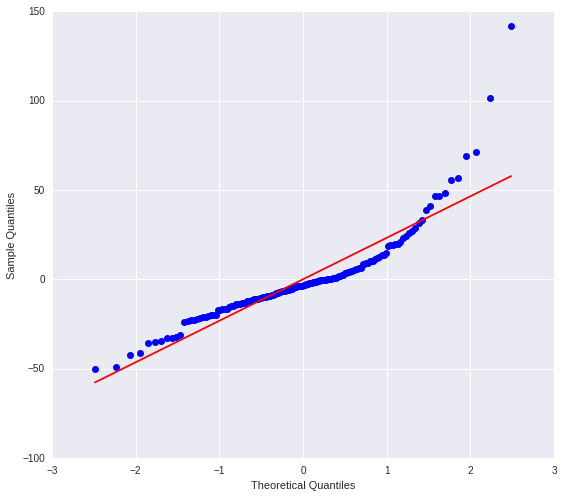
The qqplot for our regression model shows that the residuals do not follow a straight line, they start consistently above the line, then stay consistently below it, then rise above it. This behaviour indicates some degree of left skewing, showing that our residuals did not follow perfect normal distribution. There might be other explanatory variables that we might consider including in our model, that could improve our estimation.
Standardized Residuals
To evaluate the overall fit of the predicted values of the response variable to the observed values and to look for outliers, we can examine a plot of the standardized residuals for each of the observations. The standardized residuals are the residual values transformed to have a mean of zero and a standard deviation of one. In a standard normal distribution 95% of the observations are expected to fall within 2 standard deviations of the mean.
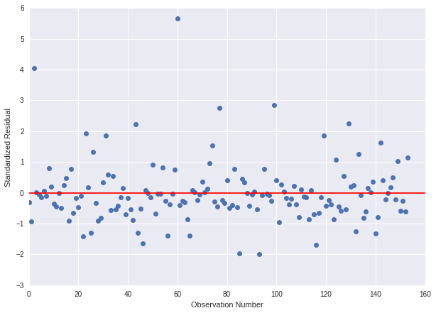
If we take a look at this plot, we see that most of the residuals fall within one standard deviation of the mean (they're either between -1 or 1), and there are six countries with residuals that are more than 2 standard deviations above or below the mean of 0. With the standard normal distribution, we would expect 95% of the values of the residuals to fall between two standard deviations of the mean. Residual values that are more than two standard deviations from the mean in either direction, are a warning sign that we may have some outliers. There are two extreme outliers that have four or more standard deviations from the mean.
Approximately 4.5% of the residuals are greater than or equal to an absolute value of 2, while 2.6% of them exceeded an absolute value of 2.5, indicating that there is evidence that the level of error within our model is unacceptable. In order to improve the fit of this model, we should include more explanatory variables to better explain the variability in our child mortality rate response variable.
Outliers and Leverage
We can examine a leverage plot to identify observations that have an unusually large influence on the estimation of the predicted value of the response variable, under-five child mortality rate, or that are outliers, or both. A point with zero leverage has no effect on the regression model. And outliers are observations with residuals greater than 2 or less than -2.
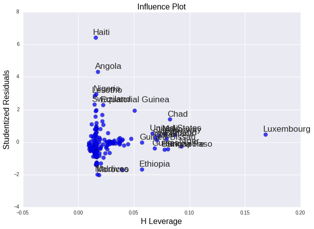
As we can see in the leverage plot, we have a few outliers, countries that have residuals greater than 2 or less than -2. This plot also tells us that these outliers have small or close to zero leverage values, meaning that although they are outlying observations, they do not have an undue influence on the estimation of the regression model. We can see that there are a few cases with relatively higher leverage, but one in particular is more obvious in terms of having an influence on the estimation of the predicted value of child mortality rate. This observation (Luxembourg) has a high leverage but is not an outlier, it is close to the 0 value of the studentized residuals . We don't have any observations that are both high leverage and outliers.
Additional Regression Diagnostic Plots
We can generate a few more plots to help us determine how specific explanatory variables contribute to the fit of our model. In this example we're examining the mean years in school for women explanatory variable.
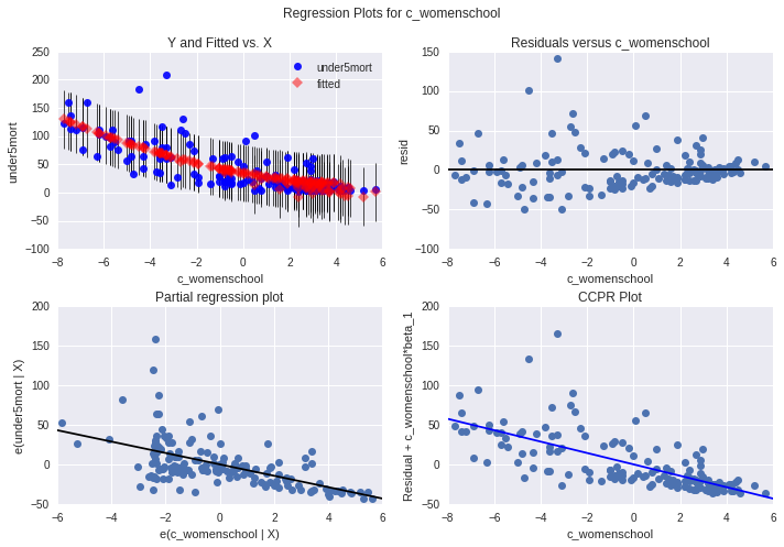
The plot in the upper right hand corner shows the residuals for each observation at different values of mean years in school for women. We can see that the absolute values of the residuals are significantly larger at lower values of the independent variable and get smaller, closer to zero, as female education rate increases. This is consistent with the other diagnostic plots that indicate that residuals are not quite randomly distributed and this confirms that the model fits poorly to the data.
The partial regression plot (ower left hand corner) shows the relationship between the response variable and the primary explanatory variable, after controlling for the other explanatory variables. When we take a look at the plot for mean years in school for women, we can see that, it shows a linear association. This suggests that female education has a statistically significant association with under-five child mortality rate, although residuals are spread out more at lower levels of female education, indicating more child mortality rate prediction error in countries with lower average schooling of women. There might be some other explanatory variables that can help us to improve our model.
Python code
# -*- coding: utf-8 -*-
# Created on 18/08/2016
# Author Ernő Gólya

%matplotlib inline
# import libraries
import pandas as pd
import numpy as np
import seaborn
import matplotlib.pyplot as plt
import statsmodels.formula.api as smf
import statsmodels.api as sm
#import statsmodels.stats.multicomp as multi

# read in data file
data = pd.read_csv('custom_gapminder_2.csv', low_memory=False)

# set variables to numeric
data["incomeperperson"] = pd.to_numeric(data["incomeperperson"],errors='coerce')
data["under5mort"] = pd.to_numeric(data["under5mort"],errors='coerce')
data["womenschool"] = pd.to_numeric(data["womenschool"],errors='coerce')
data["healthexpend"] = pd.to_numeric(data["healthexpend"],errors='coerce')

# remove observations with NaN values in any variables of interest
data = data.dropna()

# use country names as row names/indices for plotting purposes
data.index = data["country"]
data.drop("country", axis=1)

# create copy of data set
sub1 = data.copy()

# center explanatory variables
sub1['c_womenschool'] = data['womenschool'] - data['womenschool'].mean()
sub1['c_incomeperperson'] = data['incomeperperson'] - data['incomeperperson'].mean()
sub1['c_healthexpend'] = data['healthexpend'] - data['healthexpend'].mean()

# first order (linear) scatterplot
fig=plt.figure(figsize=(10, 7), dpi= 80, facecolor='w', edgecolor='k')
scat1 = seaborn.regplot(x='womenschool', y='under5mort', data=sub1, scatter=True)
plt.xlabel('Mean years of schooling for women')
plt.ylabel('Under-five mortality rate (per 1,000 live births)')
plt.title('Scatterplot for the association between Child mortality rate and Mean years of schooling for women');

# fit second order polynomial
# run the 2 scatterplots together to get both linear and second order fit lines
scat1 = seaborn.regplot(x='womenschool', y='under5mort', data=sub1, order=2, scatter=True)
plt.xlabel('Mean years of schooling for women')
plt.ylabel('Under-five mortality rate (per 1,000 live births)')
plt.title('Scatterplot for the association between Child mortality rate and Mean years of schooling for women');

# linear regression model for schooling of women and child mortality
print "OLS regression model for the association between schooling of women and child mortality rate"
model1 = smf.ols('under5mort ~ c_womenschool', data=sub1).fit()
print model1.summary()

# quadratic (polynomial) regression analysis
print "Quadratic OLS regression model for the association between schooling of women and child mortality rate"
model2 = smf.ols('under5mort ~ c_womenschool + I(c_womenschool**2)', data=sub1).fit()
print model2.summary()

# add income per person
model3 = smf.ols('under5mort ~ c_womenschool + I(c_womenschool**2) + c_incomeperperson', data=sub1).fit()
print model3.summary()

# add expenditure on health
model4 = smf.ols('under5mort ~ c_womenschool + I(c_womenschool**2) + c_healthexpend', data=sub1).fit()
print model4.summary()

# add income per person and expenditure on health
model5 = smf.ols('under5mort ~ c_womenschool + I(c_womenschool**2) + c_incomeperperson + c_healthexpend', data=sub1).fit()
print model5.summary()

# Q-Q plot for normality under5mort + c_womenschool + I(c_womenschool**2) + c_incomeperperson
fig, ax = plt.subplots(figsize=(9, 8))
fig1 = sm.qqplot(model3.resid, line = 'r', ax=ax)

# simple plot of residuals
fig=plt.figure(figsize=(10, 7), dpi= 80, facecolor='w', edgecolor='k')
stdres=pd.DataFrame(model3.resid_pearson)
plt.plot(stdres, 'o', ls='None')
l = plt.axhline(y=0, color='r')
plt.ylabel('Standardized Residual')
plt.xlabel('Observation Number');

fig, ax = plt.subplots(figsize=(10, 7))
fig3 = sm.graphics.influence_plot(model3, size=8, ax=ax)

# additional regression diagnostic plots
fig2 = plt.figure(figsize = (10, 7))
fig2 = sm.graphics.plot_regress_exog(model3,  "c_womenschool", fig=fig2)