Machine Learning for Data Analysis: Lasso Regression

LASSO (Least Absolute Shrinkage and Selection Operator) regression analysis is a supervised machine learning method for linear regression models that involves penalizing the absolute size of the regression coefficients. The goal of lasso regression is to obtain the subset of predictors that minimizes prediction error for a quantitative response variable. Penalizing the parameters (imposing a constraint on the model estimates) causes regression coefficients for some variables to shrink towards zero. The larger the penalty applied, the further estimates are shrunk towards zero. Variables with a regression coefficient equal to zero after the shrinkage process are excluded from the model. Variables with non-zero regression coefficients are most strongly associated with the response variable. This is helpful when we want some automatic feature selection, or when dealing with highly correlated predictors. When the relationship between the response variable and the predictors is linear and we have a large number of observations, then OLS regression parameter estimates will have low bias and low variance. However, if we have a relatively small number of observations and a large number of predictors, then the variance of the OLS perimeter estimates will be higher. In this case, Lasso Regression is useful because shrinking the regression coefficient can reduce variance without a significant increase in bias. Lasso Regression can also increase model interpretability, by removing unimportant variables from the model.

Running a Lasso Regression Analysis

To demonstrate how lasso regression works, let's create a model using the gapminder dataset in which our goal is to identify a set of variables that best predicts the under-five child mortality rate in a country.

The quantitative response variable measures child mortality per 1,000 live births. The response values range from 2.4 to 208.8. Quantitative predictors include mean years in school for women, per capita expenditure on health, income per person, estimated HIV prevalence, urban rate, mean age at 1st marriage of women, corruption perception index, access to improved sanitation facilities, access to improved drinking water sources, teen fertility rate and alcohol consumption.

Let's see how we test a Lasso regression model in Python. After deleting observations with missing data on any of the variables using the .dropna() function, we will have 105 countries left in our dataset. In order to have the predictive variables on the same scale (meaning that all the predictors get the same penalty), we standardize the predictors by using the preprocessing.scale() function to have a mean equal to zero and a standard deviation equal to one. Then we use the train_test_split() function to randomly split the dataset into a training dataset consisting of 70% of the total observations (N=73) and a test data set with the other 30% of the observations(N=32).

Shape of the training and test samples
(73, 11)
(32, 11)
(73,)
(32,)

LASSO Regression has a couple of different model selection algorithms. In this example, we will use the LAR Algorithm (Least Angle Regression) with the LassoLarsCV() function. This algorithm starts with no predictors in the model and adds a predictor at each step, first adding a predictor that is most correlated with the response variable and moving it towards the least score estimate until there is another predictor. Then it adds the next predictor to the model and starts the least square estimation process over again with both variables. The LAR algorithm continues with this process until it has tested all the predictors, shrinking parameter estimates and removing predictors with coefficients that have shrunk to zero. We use k-fold cross validation with ten random folds from the training dataset to select the best fitting model and obtain a more accurate estimate of our model’s test error rate by adding the cv=10 parameter to the LassoLarsCV function. The first fold of the training dataset is treated as a validation set, and the model is estimated using the remaining nine folds. At each step of the estimation process, when a new predictor is added to the model, the mean-square error for the validation fold is calculated for each of the other nine folds and then averaged. The model that produces the lowest mean-square error is selected as the best model to validate using the test dataset.

Regression coefficients of predictors

      Variable Name  Reg. Coeff
0           hivrate    6.150202
1         urbanrate   -3.667812
2       womenschool  -11.880371
3      healthexpend    2.665338
4   incomeperperson    3.432357
5          sanit_pc  -12.617347
6    watersource_pc   -2.668104
7     ageofmarriage   -2.918323
8     teenfertility    7.218451
9    alcconsumption    0.000000
10     corrupt_perc   -3.986865

Predictors with regression coefficients that do not have a value of zero are included in the selected model while variables with regression coefficients equal to zero are removed. The results show that of the 11 variables, 10 were retained in the final model, while 1 variable (alcohol consumption) was removed. During the estimation process, access to improved sanitation facilities and mean years in school for women were most strongly associated with child mortality (negative association), followed by teen fertility rate and estimated HIV prevalence showing the strongest positive relationship with the target variable. Other predictors associated with child mortality included per capita expenditure on health, income per person, urban rate, mean age at 1st marriage of women, corruption perception index and access to improved drinking water sources. These 10 variables accounted for 88.35% of the variance in the under-five mortality response variable.

Coefficient Progression

We can visualize the progression of the regression coefficients through the model selection process by plotting the change in the regression coefficient by values of the penalty parameter at each step of the selection process. The result can be seen in the graph below.

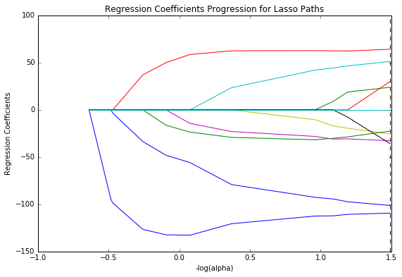
This plot shows the relative importance of the predictor selected at any step of the selection process, how the reggression coefficients changed with the addition of a new predictor at each step, as well as the steps at which each variable entered the model. As we know from the list of the regression coefficients, access to improved sanitation facilities, the blue line, has the largest (absolute) regression coefficient. It has entered into the model first, followed by mean years in school for women, the other blue line at step two, teen fertility, the red line at step three and so on.

MSE for each fold

The following plot shows the change in the mean square error for the change in the penalty parameter alpha at each step in the selection process.

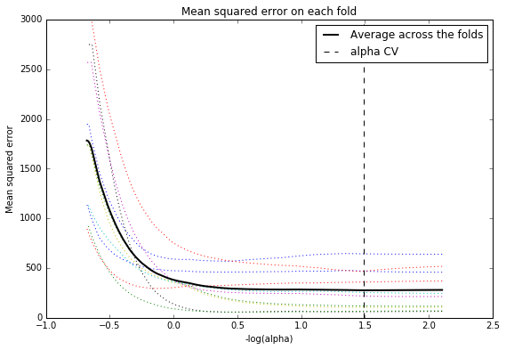
The average mean square error across all cross validation folds is plotted as the thick black line. We can see the variability across the individual cross-validation folds in the training dataset. The change in the mean square error as variables are added to the model follows the same pattern for each fold. Initially it decreases rapidly and then levels off to a point at which adding more predictors doesn't lead to much reduction in the mean square error.

MSE and R-square results

We can also calculate the average mean square error and the R-square for the proportion of variance in child mortality, that is explained by the selected model in the training set and in the test set when the selected model is applied to the test data.

Training data MSE
201.798852341

Test data MSE
811.948455593

MSE, representing the difference between the actual observations and the observation values predicted by the model, is used to determine the extent to which the model fits the data and whether the removal or some explanatory variables, simplifying the model, is possible without significantly harming the model's predictive ability. The mean square error for the test set (MSE=201.79) is much higher than that of the training set (MSE=811.94), suggesting that it is likely that the selected model badly overfit the data (we have created a model that tests well in sample, but has little predictive value when tested out of sample). The selected model is less accurate in predicting under-five mortality in the test data.

Given the fact that the sample dataset is fairly small (105 observations), including 11 predictors in the model considerably increases it's complexity. The new more complicated function "overfits" the data, and the complex overfitted model will likely perform worse on validation data outside the training dataset. If some variables are removed, we may get a different output which may have a better test mean squared error.

Training data R-square
0.883500155514

Test data R-square
0.649046008446

The R-square values are 0.88 and 0.64, indicating that the selected model explained 88% and 64% of the variance in child mortality for the training and test sets, respectively. We can see hat the model we obtained from the training dataset could explain 64% of the child mortality rate variance for the countries in the test dataset.

Python code

# -*- coding: utf-8 -*-
#
# Created on Sept 01 2016
# @author: Ernő Gólya

%matplotlib inline
import pandas as pd
import numpy as np
import matplotlib.pylab as plt
from sklearn.cross_validation import train_test_split
from sklearn.linear_model import LassoLarsCV
from sklearn import preprocessing
from sklearn.metrics import mean_squared_error

# data management
data = pd.read_csv("custom_gapminder_3.csv")

variables = ['under5mort', 'womenschool', 'healthexpend', 'incomeperperson', 'hivrate', 'urbanrate',
           'ageofmarriage', 'corrupt_perc', 'sanit_pc', 'watersource_pc', 'teenfertility', 'alcconsumption']

data = data[variables]

# convert selected variables to numeric
for variable in variables:
    data[variable] = pd.to_numeric(data[variable],errors='coerce')

# delete observations with missing value(s)
data1 = data.dropna()
data2 = data1.copy()

# create list of predictors
pred_variables = [n for n in variables if n != 'under5mort']

# standardize predictors to have mean=0 and sd=1
for feature in pred_variables:
    data2[feature] = preprocessing.scale(data2[feature].astype('float64'))

# create separate data sets for predictor variables and target variable
predictors = data2[pred_variables]
targets = data2.under5mort

# split dataset into training and testing sets
pred_train, pred_test, tar_train, tar_test  =   train_test_split(predictors, targets, test_size=0.3, random_state=123)

# specify the lasso regression model
model = LassoLarsCV(cv=10, precompute=False).fit(pred_train,tar_train)

# print variable names and regression coefficients
d = dict(zip(predictors.columns, model.coef_))
print "{:<20} {:<25}".format('Variable Name','Regression Coefficient')
for k, v in d.items():
    num = v
    print "{:<20} {:<25}".format(k, num)

# another way to print variable names and regression coefficients
rc_data = pd.DataFrame(d.items(), columns=['Variable Name', 'Reg. Coeff'])
print rc_data

# plot coefficient progression
m_log_alphas = -np.log10(model.alphas_)
fig=plt.figure(figsize=(9, 6))
plt.plot(m_log_alphas, model.coef_path_.T)
plt.axvline(-np.log10(model.alpha_), linestyle='--', color='k', label='alpha CV')
plt.ylabel('Regression Coefficients')
plt.xlabel('-log(alpha)')
plt.title('Regression Coefficients Progression for Lasso Paths');

# plot mean square error for each fold
m_log_alphascv = -np.log10(model.cv_alphas_)
plt.figure(figsize=(9, 6))
plt.plot(m_log_alphascv, model.cv_mse_path_, ':')
plt.plot(m_log_alphascv, model.cv_mse_path_.mean(axis=-1), 'k', label='Average across the folds', linewidth=2)
plt.axvline(-np.log10(model.alpha_), linestyle='--', color='k', label='alpha CV')
plt.legend()
plt.xlabel('-log(alpha)')
plt.ylabel('Mean squared error')
plt.title('Mean squared error on each fold');

# MSE from training and test data
train_error = mean_squared_error(tar_train, model.predict(pred_train))
test_error = mean_squared_error(tar_test, model.predict(pred_test))
print 'Training data MSE'
print train_error
print '\nTest data MSE'
print test_error

# R-square from training and test data
rsquared_train = model.score(pred_train, tar_train)
rsquared_test = model.score(pred_test, tar_test)
print 'Training data R-square'
print rsquared_train
print '\nTest data R-square'
print rsquared_test

# print sape of training and test samples
print "Shape of the training and test samples"
print pred_train.shape
print pred_test.shape
print tar_train.shape
print tar_test.shape