Hypothesis Testing and ANOVA
h 01 augusztus 2016 by Ernő GólyaThis is part of my coursework for the Data Analysis Tools course by Wesleyan University on Coursera. Week 1 assignment is to run an analysis of variance. Analyze and interpret post hoc paired comparisons in instances where the original statistical test was significant, and we were examining more than two groups. Data source: Gapminder World.
Original research question: What is the correlation between child mortality and female education?
After selecting a data set and research question, managing our variables of interest and visualizing their relationship graphically (Data Management and Visualization coursework), it is time to test those relationships statistically. The first assignment deals with analysis of variance. Analysis of variance assesses whether the means of two or more groups are statistically different from each other. This analysis is appropriate whenever we want to compare the means (quantitative variables) of groups (categorical variables). The null hypothesis is that there is no difference in the mean of the quantitative variable across groups (categorical variable), while the alternative is that there is a difference.
Null Hypothesis: There is no association between the average amount of time (years) women spend in schools and the under-five child mortality rate in a country.
Alternate Hypothesis: There is an association between the average amount of time (years) women spend in schools and the under-five child mortality rate in a given country.
Categorizing the explanatory variable
Both response variable (under-five child mortality per 1,000 live births) and explanatory variable (mean years of schooling for women) are quantitative variables. In order to perform an Analysis of Variance (ANOVA) test, I had to create categories for the explanatory variable (womenschool -> womenschool_cat): 0-4 years, 4-8 years, 8-12 years, 12-16 years.
Model Interpretation for ANOVA
When examining the association between under-five child mortality rate (quantitative response) and mean years of schooling for women categories, an Analysis of Variance (ANOVA) revealed that there are significant differencies in child mortality rates among countries that fell into different categories of average years of schooling for women (see graph for visual presentation and OLS regression results below).
Means for under5mort by Schooling of Women
womenschool_cat under5mort
0-4 years 104.822222
4-8 years 68.517647
8-12 years 23.855882
12-16 years 8.132353
Standard deviations for under5mort by Schooling of Women
womenschool_cat under5mort
0-4 years 29.084574
4-8 years 45.223790
8-12 years 21.431358
12-16 years 5.206739
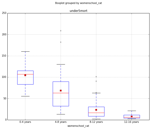
Countries with higher female education scores demonstrated lower child mortality rate with an F(3, 150) = 68.49 and a p-value of 5.92e-28. The probability of the between-categories mean square being 68.49 times the within-categories mean square, if the null hypothesis is true, is p<.0001.
The p-value is well below our significance level of 0.05. It would be quite unlikely to have F-value this large if there were no real difference among the means. Therefore it implies that we can reject the null hypothesis and take on the alternate hypothesis as valid, concluding that child mortality rate and the level of female education are significantly associated.
                                OLS Regression Results
    ==============================================================================
    Dep. Variable:             under5mort   R-squared:                       0.578
    Model:                            OLS   Adj. R-squared:                  0.570
    Method:                 Least Squares   F-statistic:                     68.49
    Date:                Mon, 01 Aug 2016   Prob (F-statistic):           5.92e-28
    Time:                        11:19:18   Log-Likelihood:                -726.94
    No. Observations:                 154   AIC:                             1462.
    Df Residuals:                     150   BIC:                             1474.
    Df Model:                           3
    Covariance Type:            nonrobust
    =====================================================================================================
                                            coef    std err          t      P>|t|      [95.0% Conf. Int.]
    -----------------------------------------------------------------------------------------------------
    Intercept                           104.8222      6.485     16.164      0.000        92.009   117.635
    C(womenschool_cat)[T.4-8 years]     -36.3046      8.020     -4.527      0.000       -52.151   -20.459
    C(womenschool_cat)[T.8-12 years]    -80.9663      7.293    -11.102      0.000       -95.376   -66.557
    C(womenschool_cat)[T.12-16 years]   -96.6899      8.020    -12.057      0.000      -112.536   -80.844
    ==============================================================================
    Omnibus:                       67.145   Durbin-Watson:                   2.205
    Prob(Omnibus):                  0.000   Jarque-Bera (JB):              276.775
    Skew:                           1.595   Prob(JB):                     7.93e-61
    Kurtosis:                       8.741   Cond. No.                         6.98
    ==============================================================================

    Warnings:
    [1] Standard Errors assume that the covariance matrix of the errors is correctly specified.
Model Interpretation for post hoc ANOVA results
ANOVA revealed that the categories for the explanatory variable were significantly associated to the quantitative response variable. This rules out the null hypothesis that the variables are no different (all means equal) and shows that there is, in fact, a difference between the means. As the ANOVA test shows that the means aren’t all equal, our next step is to determine which means are different, to our level of significance.
The post hoc comparisons of mean (performed through the Tukey HSD test) shows all comparisons reporting statistically significant difference. In every case the reject = True result implies that we can disapprove the null hypothesis for the education levels compared to each other and accept the alternate hypothesis that group means are significantly different.
        Multiple Comparison of Means - Tukey HSD,FWER=0.05
    ==========================================================
       group1      group2   meandiff   lower    upper   reject
    ----------------------------------------------------------
     0-4 years  12-16 years -96.6899 -117.5267 -75.853   True
     0-4 years   4-8 years  -36.3046  -57.1414 -15.4677  True
     0-4 years   8-12 years -80.9663  -99.9144 -62.0183  True
    12-16 years  4-8 years  60.3853    43.048  77.7226   True
    12-16 years  8-12 years 15.7235    0.709   30.7381   True
     4-8 years   8-12 years -44.6618  -59.6763 -29.6472  True
    ----------------------------------------------------------
Python source code
# -*- coding: utf-8 -*-
# Created on 01/08/2016
# Author Ernő Gólya

%matplotlib inline
# Import libraries
import pandas as pd
import numpy as np
import matplotlib.pyplot as plt
import statsmodels.formula.api as smf
import statsmodels.stats.multicomp as multi

# Reading in data file
data = pd.read_csv('custom_gapminder_2.csv', low_memory=False)

# Setting variables to numeric
data["incomeperperson"] = pd.to_numeric(data["incomeperperson"],errors='coerce')
data["under5mort"] = pd.to_numeric(data["under5mort"],errors='coerce')
data["womenschool"] = pd.to_numeric(data["womenschool"],errors='coerce')
data["healthexpend"] = pd.to_numeric(data["healthexpend"],errors='coerce')

# Remove observations with NaN values in any variables of interest
# Describe function returns NaN for percentiles if dataset contains NaN
data = data.dropna()

# Creating categories for quantitative variables
data["incomeperperson_cat"] = pd.cut(data.incomeperperson, [1, 1000, 4000, 12000, 65000], labels=["Low", "Lower middle", "Upper middle", "High" ])
data["under5mort_cat"] = pd.cut(data.under5mort, [1, 40, 80, 120, 160, 220], labels=["0-40","40-80", "80-120", "120-160", "160-220"])
data["womenschool_cat"] = pd.cut(data.womenschool, [0, 4, 8, 12, 16], labels=["0-4 years", "4-8 years", "8-12 years", "12-16 years"])
data["healthexpend_cat"] = pd.cut(data.healthexpend, [1, 500, 1000, 2000, 5000, 9000], labels=["1-500", "500-1000", "1000-2000", "2000-5000", "5000-9000"])

# Creating subgrup for child mortality (quantitative) and mean years in school (categories)
sub1 = data[['under5mort', 'womenschool_cat']]

# Show frequency table for mean years in school categories
print "Frequency table for Schooling of Women"
c1 = sub1.groupby('womenschool_cat').size()
print c1
print ""

# Using ols function for calculating the F-statistic and associated p value
model1 = smf.ols(formula='under5mort ~ C(womenschool_cat)', data=sub1)
result1 = model1.fit()
print result1.summary()
print ""

# Print means
print "Means for under5mort by Schooling of Women"
m1= sub1.groupby('womenschool_cat').mean()
print m1
print ""

# Print standard deviations
print "Standard deviations for under5mort by Schooling of Women"
sd1= sub1.groupby('womenschool_cat').std()
print sd1
print ""

# Perform post-hoc analysis
mc1 = multi.MultiComparison(sub1['under5mort'], sub1['womenschool_cat'])
result2 = mc1.tukeyhsd()
print result2.summary()

# Plotting bivariate distributions
sub1.boxplot(column='under5mort', by='womenschool_cat', grid=True, figsize=(10, 8), layout=None, showmeans=True);