Machine Learning for Data Analysis: Decision Trees
p 26 augusztus 2016 by Ernő GólyaMachine learning encompasses a wide range of statistical methods that can be used to describe associations, search for patterns, or make predictions about outcomes from a set of inputs. When our goal is to predict the value of a response variable based on a number of predictors, then we are using a supervised learning approach. We use a subset of observations from our dataset (training set), to learn about the data and then test the model we get on a different set of observations (test set). When we apply our statistical model to the test set, we're interested in the accuracy of our model, that can be assessed by the test error rate, which is a measure of the extent to which a model correctly classifies observations into categories. Our goal then is to identify a model that minimizes the test error rate.
Decision Trees
Decision tree is a type of supervised learning algorithm that is mostly used in classification problems. It is a type of data mining method that allows us to explore the presence of potentially complicated interactions within our data by creating subgroups (or segmentations) by applying a series of rules over and over again, which choose variable arrangements that best predict the target variable. It works for both categorical and continuous input and output variables. When the response variable is categorical, the model is called a classification tree. Decision trees are so-named because the predictive model can be represented in a tree-like structure in which each internal node represents a test on a variable (a split based on the values of one of the explanatory variables), each branch represents the outcome of the test and each leaf node represents a class or subgroup based on the combination of previous splits.
About the Data
The dataset is compiled from data available on the Gapminder website. This data sample provides values for under-five child mortality rate (target variable), mean years in school for women, per capita total expenditure on health, income per person, estimated HIV prevalence, urban population rate, mean age at 1st marriage of women, corruption perception index, access to improved sanitation facilities, access to improved drinking water sources and teen fertility rate (explanatory variables or predictors) for 167 countries from years between 2005 and 2010. After removing countries with missing data (all variables examined) there are 106 observations left.
The response variable (child mortality rate) is a quantitative variable, so for this analysis it is converted into a binary categorical variable (u5_abovemedian), using the global median of the under5mort variable as a cut-point.
u5_abovemedian
0: under5mort <= median of U5MR rates of all countries in dataset
1: under5mort > median of U5MR rates of all countries in dataset
Because decision tree analyses cannot handle any NA's in our dataset, we need to create a data frame that drops all NA's. We can take a look at various characteristics of our data by using the d types and describe functions to examine data types and summary statistics*, and include the train test split function for predictors and target. Size ratio is set to 60% for the training sample and 40% for the test sample. The training sample has 67 observations, and 8 explanatory variables. The test sample has 45 observations and again 8 explanatory variables.
Shape of the training and test samples
(67, 8)
(45, 8)
(67,)
(45,)
Running a Classification Tree
Decision tree analysis was performed to test nonlinear relationships among a series of explanatory variables and a binary, categorical response variable. All possible separations or cut-points are tested and the separation yielding the minimum impurity or error is selected, and subgroups showing similar outcomes but different explanatory variable combinations are generated. The following explanatory variables were included as possible contributors to a classification tree model evaluating under-five child mortality (response variable): mean years in school for women, income per person, estimated HIV prevalence, urban rate, mean age at 1st marriage of women, access to improved sanitation facilities, access to improved drinking water sources and teen fertility rate. The following image is the decision tree that our model generated on the training set.
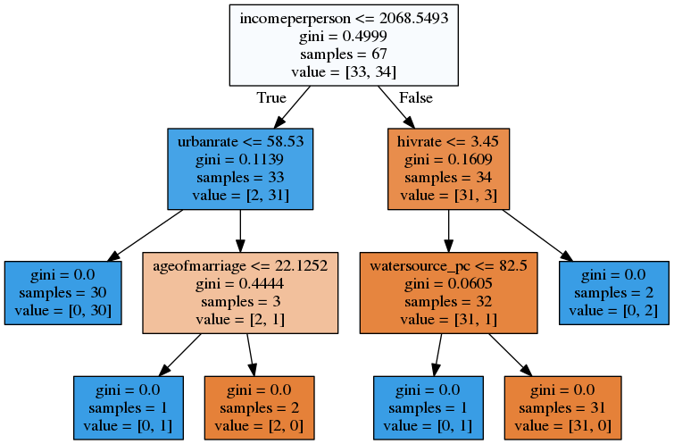
The resulting tree starts with the split on income per person. If the value for income per person is less than or equal to 2068.54, then the observations move to the left side of the split and include 33 of the 67 countries in the training sample. From this node, another split is made on urban rate, such that among those 33 countries on the left side, 30 countries reported 58.53% or less urban rate while only 3 are above that level. To the left of that split we see that all the 30 countries have child mortality above the global median. To the right of that split a further subdivision was made with the age of first marriage variable. Here 1 country has ageofmarriage <= 22.12 years value, and has child mortality above the world average. On the other hand, those countries above 22.12 years of age of marriage are below the global median child mortality rate.
Following down the right side of the tree, we can see that child mortality rate is below the global average in those countries where HIV rate <= 3.45 and access to improved drinking water sources is above 82.5%. Countries with larger HIV rate or hivrate <= 3.45 but below the cutoff point (82.5) of improved drinking water sources are more likely to have under-five mortality rate above the average.
Model Accuracy
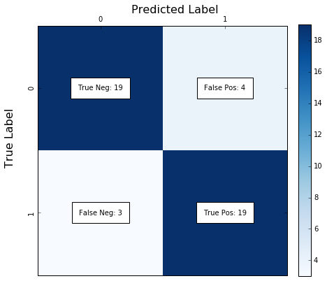
The confusion matrix shows the correct and incorrect classifications of our decision tree. The diagonal 19 and 19 represents the number of true negative for child mortality, and the number of true positives, respectively. The 3, on the bottom left, represents the number of false negatives, classifying countries with child mortality above the global average as countries below the median. The number of false positives on the top right is 4, classifying a country as having child mortality rate above the average while it isn't.
Confusion matrix
[[19  4]
 [ 3 19]]

Accuracy score
0.844444444444
The accuracy score is approximately 0.84, which suggests that the decision tree model has classified 84% of the sample correctly.
Confusion Matrix
Python code
# -*- coding: utf-8 -*-
"""
Created on Aug 24 2016
@author: Ernő Gólya
"""
from pandas import Series, DataFrame
import pandas as pd
import numpy as np
import os
import matplotlib.pylab as plt
from sklearn.cross_validation import train_test_split
from sklearn.tree import DecisionTreeClassifier
from sklearn.metrics import classification_report
import sklearn.metrics

#pd.set_option('display.float_format', lambda x:'%f'%x)

inp_data = pd.read_csv("custom_gapminder_3.csv")

inp_data1 = inp_data[['under5mort',
                     'womenschool',
                     'incomeperperson',
                     'hivrate',
                     'urbanrate',
                     'ageofmarriage',
                     'sanit_pc',
                     'watersource_pc',
                     'teenfertility']]

data = inp_data1.copy()

data["incomeperperson"] = pd.to_numeric(data["incomeperperson"],errors='coerce')
data["under5mort"] = pd.to_numeric(data["under5mort"],errors='coerce')
data["womenschool"] = pd.to_numeric(data["womenschool"],errors='coerce')
data["hivrate"] = pd.to_numeric(data["hivrate"],errors='coerce')
data["urbanrate"] = pd.to_numeric(data["urbanrate"],errors='coerce')
data["ageofmarriage"] = pd.to_numeric(data["ageofmarriage"],errors='raise')
data["sanit_pc"] = pd.to_numeric(data["sanit_pc"],errors='raise')
data["watersource_pc"] = pd.to_numeric(data["watersource_pc"],errors='raise')
data["teenfertility"] = pd.to_numeric(data["teenfertility"],errors='raise')

data2 = data.dropna()

# create u5_abovemedian variable (value = 1 if under5mort > under5median, othervise value = 0)
under5median = data2['under5mort'].median()
def u5_abovemedian(row):
    if row['under5mort'] > under5median:
        return 1
    else:
        return 0
data3 = data2.copy()
data3['u5_abovemedian'] = data3.apply(lambda row: u5_abovemedian(row), axis=1)

predictors = data3[['womenschool',
 'incomeperperson',
 'hivrate',
 'urbanrate',
 'ageofmarriage',
 'sanit_pc',
 'watersource_pc',
 'teenfertility']]
targets = data3.u5_abovemedian
pred_train, pred_test, tar_train, tar_test  =   train_test_split(predictors, targets, test_size=.4)

print "Shape of the training and test samples"
print pred_train.shape
print pred_test.shape
print tar_train.shape
print tar_test.shape

classifier = DecisionTreeClassifier()
classifier = classifier.fit(pred_train,tar_train)

predictions = classifier.predict(pred_test)

print "\nConfusion matrix"
cm = sklearn.metrics.confusion_matrix(tar_test, predictions)
print cm
print "\nAccuracy score"
print sklearn.metrics.accuracy_score(tar_test, predictions)

from sklearn import tree
from io import BytesIO as StringIO
from IPython.display import Image
from IPython import display
out = StringIO()
tree.export_graphviz(classifier, out_file=out, feature_names=['womenschool',
 'incomeperperson',
 'hivrate',
 'urbanrate',
 'ageofmarriage',
 'sanit_pc',
 'watersource_pc',
 'teenfertility'], filled=True)
import pydotplus
graph = pydotplus.graph_from_dot_data(out.getvalue())
display.Image(graph.create_png())

print data3.dtypes
print "\nDescription of variables"
data3[['under5mort', 'womenschool', 'incomeperperson', 'hivrate', 'urbanrate']].describe()
data3[['u5_abovemedian', 'ageofmarriage', 'sanit_pc', 'watersource_pc', 'teenfertility']].describe()
*Description of Variables
under5mort         float64
womenschool        float64
incomeperperson    float64
hivrate            float64
urbanrate          float64
ageofmarriage      float64
sanit_pc           float64
watersource_pc     float64
teenfertility      float64
u5_abovemedian       int64
dtype: object

       under5mort  womenschool  incomeperperson     hivrate   urbanrate
count  112.000000   112.000000       112.000000  112.000000  112.000000
mean    42.924107     8.683929      7625.846701    2.221161   53.821964
std     43.080591     3.566954     11702.931523    4.929565   22.559999
min      2.400000     1.300000       115.305996    0.060000   10.400000
25%      8.125000     5.700000       554.610504    0.100000   36.835000
50%     24.250000     9.150000      1918.152900    0.400000   56.580000
75%     65.125000    11.900000      6335.202562    1.300000   70.545000
max    208.800000    14.700000     52301.587179   25.900000  100.000000

       u5_abovemedian  ageofmarriage    sanit_pc  watersource_pc  \
count      112.000000     112.000000  112.000000      112.000000
mean         0.500000      23.909548   69.196429       86.419643
std          0.502247       3.694327   31.640959       15.724909
min          0.000000      17.600199    9.000000       40.000000
25%          0.000000      21.240263   39.000000       79.750000
50%          0.500000      22.995199   81.000000       92.000000
75%          1.000000      26.569345   99.000000       99.000000
max          1.000000      33.202919  100.000000      100.000000

       teenfertility
count     112.000000
mean       53.729405
std        43.758964
min         4.000000
25%        15.375000
50%        43.000000
75%        76.000000
max       199.000000