Chi-Square Test of Independence
k 02 augusztus 2016 by Ernő GólyaThis is part of my coursework for the Data Analysis Tools course by Wesleyan University on Coursera. Week 2 assignment: Run a Chi-Square Test of Independence. Analyze and interpret post hoc paired comparisons in instances where the original statistical test was significant, and we were examining more than two groups.
Data source: Gapminder World.
This assignment deals with the Chi-Square Test of Independence. A Chi-Square Test of Independence compares frequencies of one categorical variable for different values of a second categorical variable. The null hypothesis is that the relative proportions of one variable are independent of the second variable. The alternate hypothesis is that the relative proportions of one variable are associated with the second variable.
I'am interested in whether there is a relationship between the income level and the under-5 child mortality rate (U5MR) of a country. More specifically I want to analyze how the proportion of the countries with a value of under-five child mortality rate above the global median (19.5) varies among the World Bank income groups (low, lower-middle, upper-middle, and high) of countries.
As the child mortality frequency distribution of the countries is skewed to the right I will use the global median of the under5mort variable for the comparison.
Null Hypothesis: There is no association between the income level category and the under-five child mortality rate in a country being higher (or lower) than the median of all countries.
Alternate Hypothesis: There is an association between the income level category and the under-five child mortality rate in a country being higher (or lower) than the median of all countries.
Categorizing the variables
The data set contains 154 countries. Both under5mort and incomeperperson are quantitative variables. In order to be able to run a Chi-Square Test I create categories for these indicators.
incomeperperson_cat:
low: 1-1,005 US$
lower-middle: 1,006-3,975 US$
upper-middle: 3,976-12,275 US$
high: > 12,275 US$
u5_abovemedian:
0: under5mort <= 19.5 (median of U5MR rates of 154 countries)
1: under5mort > 19.5 (median of U5MR rates of 154 countries)
Model Interpretation for Chi-Square Test
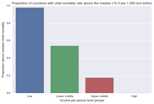
When examining the association between under-five child mortality, represented as "u5_abovemedian" (categorical response) and GDP level of country, represented as "incomeperperson_cat" (categorical explanatory), a chi-square test of independence revealed that among 154 countries in the data set, those with high GDP per capita having no under-five child mortality rate above the average (median) value of all the countries (0.00 %), compared to countries in the upper-middle income group (17.24%), lower-middle income group (54%) or low income group (97.8%), X2=83.85, df=3, p=4.5694326276298282e-18.
The low p-value suggests that there is association between the two variables. By running post hoc Chi-Square tests we can find in which comparisons we can reject the null hypothesis.
The df or degree of freedom we record is the number of levels of the explanatory variable -1. Here the df is 3 income per person which has 4 levels (df 4-1=3).
Contingency table
incomeperperson_cat  Low  Lower middle  Upper middle  High
u5_abovemedian
0                      1            23            24    29
1                     45            27             5     0
Observed counts
incomeperperson_cat       Low  Lower middle  Upper middle  High
u5_abovemedian
0                    0.021739          0.46      0.827586   1.0
1                    0.978261          0.54      0.172414   0.0
Chi-Square test
chi-square value, p value, expected counts
(83.855232383808101, 4.5694326276298282e-18, 3, array([[ 23. ,  25. ,  14.5,  14.5],
       [ 23. ,  25. ,  14.5,  14.5]]))
Factor plot for the variables
Model Interpretation for post hoc Chi-Square Test results
A Chi-Square test of independence revealed that among 154 countries the income per person level of the country and under-five child mortality rate were significantly associated, X2=83.85, df=3, p=4.5694326276298282e-18.
Post hoc comparisons of GDP levels, by pairs of under-five mortality categories revealed that countries with higher GDP per capita reported lower score of child mortality. The negative relationship between income level and child mortality was proven in almost all of the comparison tests (the p value in almost each test was lower than 0.008, i.e. p value after the Bonferroni correction) with one exception. Child mortality rate was statistically similar between the Upper middle and High income groups (X2=3.5, df=1, p=0.06).
Bonferroni adjusted p-value for 6 comparisons: p = 0.05/6 = 0.008.
    Contingency table
    COMPLvLm        Low  Lower middle
    u5_abovemedian
    0                 1            23
    1                45            27

    Observed counts
    COMPLvLm             Low  Lower middle
    u5_abovemedian
    0               0.021739          0.46
    1               0.978261          0.54

    Chi-Square test
    chi-square value, p value, expected counts
    (22.260869565217391, 2.3800765057438958e-06, 1, array([[ 11.5,  12.5],
           [ 34.5,  37.5]]))
    Contingency table
    COMPLvUm        Low  Upper middle
    u5_abovemedian
    0                 1            24
    1                45             5

    Observed counts
    COMPLvUm             Low  Upper middle
    u5_abovemedian
    0               0.021739      0.827586
    1               0.978261      0.172414

    Chi-Square test
    chi-square value, p value, expected counts
    (48.414074212893553, 3.4508262281508998e-12, 1, array([[ 15.33333333,   9.66666667],
           [ 30.66666667,  19.33333333]]))
    Contingency table
    COMPLvH         High  Low
    u5_abovemedian
    0                 29    1
    1                  0   45

    Observed counts
    COMPLvH         High       Low
    u5_abovemedian
    0                1.0  0.021739
    1                0.0  0.978261

    Chi-Square test
    chi-square value, p value, expected counts
    (66.906390554722634, 2.8471045701472532e-16, 1, array([[ 11.6,  18.4],
           [ 17.4,  27.6]]))
    Contingency table
    COMPLmvUm       Lower middle  Upper middle
    u5_abovemedian
    0                         23            24
    1                         27             5

    Observed counts
    COMPLmvUm       Lower middle  Upper middle
    u5_abovemedian
    0                       0.46      0.827586
    1                       0.54      0.172414

    Chi-Square test
    chi-square value, p value, expected counts
    (8.8223760775862043, 0.0029755895248322777, 1, array([[ 29.74683544,  17.25316456],
           [ 20.25316456,  11.74683544]]))
    Contingency table
    COMPLmvH        High  Lower middle
    u5_abovemedian
    0                 29            23
    1                  0            27

    Observed counts
    COMPLmvH        High  Lower middle
    u5_abovemedian
    0                1.0          0.46
    1                0.0          0.54

    Chi-Square test
    chi-square value, p value, expected counts
    (21.451315330582574, 3.6292697947721256e-06, 1, array([[ 19.08860759,  32.91139241],
           [  9.91139241,  17.08860759]]))
    Contingency table
    COMPUmvH        High  Upper middle
    u5_abovemedian
    0                 29            24
    1                  0             5

    Observed counts
    COMPUmvH        High  Upper middle
    u5_abovemedian
    0                1.0      0.827586
    1                0.0      0.172414

    Chi-Square test
    chi-square value, p value, expected counts
    (3.5018867924528303, 0.06129895419397504, 1, array([[ 26.5,  26.5],
           [  2.5,   2.5]]))
Python source code
# -*- coding: utf-8 -*-
# Created on 02/08/2016
# Author Ernő Gólya

%matplotlib inline
# import libraries
import pandas as pd
import numpy as np
import scipy.stats
import seaborn
import matplotlib.pyplot as plt

# read in data file
data = pd.read_csv('custom_gapminder_2.csv', low_memory=False)

# set variables to numeric
data["incomeperperson"] = pd.to_numeric(data["incomeperperson"],errors='coerce')
data["under5mort"] = pd.to_numeric(data["under5mort"],errors='coerce')
data["womenschool"] = pd.to_numeric(data["womenschool"],errors='coerce')
data["healthexpend"] = pd.to_numeric(data["healthexpend"],errors='coerce')

# remove observations with NaN values in any variables of interest
data = data.dropna()

# create categories for quantitative variable
data["incomeperperson_cat"] = pd.cut(data.incomeperperson, [1, 1005, 3975, 12275, 65000], labels=["Low", "Lower middle", "Upper middle", "High" ])

# create subgrup for child mortality (quantitative) and income per person levels (categorical)
sub1 = data[['country','under5mort', 'incomeperperson_cat']]

# create copy of subset
sub2 = sub1.copy()

# median global child mortality
under5median = sub1['under5mort'].median()

# create u5_abovemedian variable (value = 1 if under5mort > under5median, othervise value = 0)
def u5_abovemedian(row):
    if row['under5mort'] > under5median:
        return 1
    else:
        return 0
sub2['u5_abovemedian'] = sub2.apply(lambda row: u5_abovemedian(row), axis=1)

print "Global median of under-5 mortality rate is: %r" %under5median
# Global median of under-5 mortality rate is: 19.5

# contingency table of observed counts
ct1 = pd.crosstab(sub2['u5_abovemedian'], sub2['incomeperperson_cat'])
print "Contingency table\n"
print ct1,"\n\n"

# column percentages
colsum = ct1.sum(axis=0)
colpct = ct1/colsum
print "Observed counts\n"
print colpct,"\n\n"

# chi-square
print "Chi-Square test\n"
print 'chi-square value, p value, expected counts'
cs1 = scipy.stats.chi2_contingency(ct1)
print cs1

# graph percent with child mortality within each income level group
seaborn.factorplot(x="incomeperperson_cat", y="u5_abovemedian", data=sub2, kind="bar", ci=None, aspect=1.5, size=5)
plt.xlabel('Income per person level groups')
plt.ylabel('Proportion above median child mortality')
plt.title('Proportion of countries with child mortality rate above the median (19.5 per 1,000 live births)');

recode1 = {"Low": "Low", "Lower middle": "Lower middle"}
sub2['COMPLvLm'] = sub2['incomeperperson_cat'].map(recode1)

# contingency table of observed counts
ct2 = pd.crosstab(sub2['u5_abovemedian'], sub2['COMPLvLm'])
print "Contingency table\n"
print ct2,"\n\n"

# column percentages
colsum = ct2.sum(axis=0)
colpct = ct2/colsum
print "Observed counts\n"
print colpct,"\n\n"

# chi-square
print "Chi-Square test\n"
print 'chi-square value, p value, expected counts'
cs2 = scipy.stats.chi2_contingency(ct2)
print cs2

recode2 = {"Low": "Low", "Upper middle": "Upper middle"}
sub2['COMPLvUm'] = sub2['incomeperperson_cat'].map(recode2)

# contingency table of observed counts
ct3 = pd.crosstab(sub2['u5_abovemedian'], sub2['COMPLvUm'])
print "Contingency table\n"
print ct3,"\n\n"

# column percentages
colsum = ct3.sum(axis=0)
colpct = ct3/colsum
print "Observed counts\n"
print colpct,"\n\n"

# chi-square
print "Chi-Square test\n"
print 'chi-square value, p value, expected counts'
cs3 = scipy.stats.chi2_contingency(ct3)
print cs3

recode3 = {"Low": "Low", "High": "High"}
sub2['COMPLvH'] = sub2['incomeperperson_cat'].map(recode3)

# contingency table of observed counts
ct4 = pd.crosstab(sub2['u5_abovemedian'], sub2['COMPLvH'])
print "Contingency table\n"
print ct4,"\n\n"

# column percentages
colsum = ct4.sum(axis=0)
colpct = ct4/colsum
print "Observed counts\n"
print colpct,"\n\n"

# chi-square
print "Chi-Square test\n"
print 'chi-square value, p value, expected counts'
cs4 = scipy.stats.chi2_contingency(ct4)
print cs4

recode4 = {"Lower middle": "Lower middle", "Upper middle": "Upper middle"}
sub2['COMPLmvUm'] = sub2['incomeperperson_cat'].map(recode4)

# contingency table of observed counts
ct5 = pd.crosstab(sub2['u5_abovemedian'], sub2['COMPLmvUm'])
print "Contingency table\n"
print ct5,"\n\n"

# column percentages
colsum = ct5.sum(axis=0)
colpct = ct5/colsum
print "Observed counts\n"
print colpct,"\n\n"

# chi-square
print "Chi-Square test\n"
print 'chi-square value, p value, expected counts'
cs5 = scipy.stats.chi2_contingency(ct5)
print cs5

recode5 = {"Lower middle": "Lower middle", "High": "High"}
sub2['COMPLmvH'] = sub2['incomeperperson_cat'].map(recode5)

# contingency table of observed counts
ct6 = pd.crosstab(sub2['u5_abovemedian'], sub2['COMPLmvH'])
print "Contingency table\n"
print ct6,"\n\n"

# column percentages
colsum = ct6.sum(axis=0)
colpct = ct6/colsum
print "Observed counts\n"
print colpct,"\n\n"

# chi-square
print "Chi-Square test\n"
print 'chi-square value, p value, expected counts'
cs6 = scipy.stats.chi2_contingency(ct6)
print cs6

recode6 = {"Upper middle": "Upper middle", "High": "High"}
sub2['COMPUmvH'] = sub2['incomeperperson_cat'].map(recode6)

# contingency table of observed counts
ct7 = pd.crosstab(sub2['u5_abovemedian'], sub2['COMPUmvH'])
print "Contingency table\n"
print ct7,"\n\n"

# column percentages
colsum = ct7.sum(axis=0)
colpct = ct7/colsum
print "Observed counts\n"
print colpct,"\n\n"

# chi-square
print "Chi-Square test\n"
print 'chi-square value, p value, expected counts'
cs7 = scipy.stats.chi2_contingency(ct7)
print cs7