Regression Modeling in Practice: Basic Linear Regression Model
h 15 augusztus 2016 by Ernő GólyaSo far, in the Data Analysis and Interpretation Specialization courses by Wesleyan University, I have statistically tested the association between the level of female education (primary explanatory variable) and under-five child mortality rate (response variable).
This time I will test and interpret this relationship using basic linear regression analysis for the two variable.
Simple linear regression is a statistical method that allows us to describe data and explain the relationship between two quantitative variables: 1. It might be used to identify the strength of the effect that the independent variable have on a dependent variable. 2. It can be used to forecast effects or impacts of changes. Regression analysis can help us to understand how much will the dependent variable change, when we change the independent variable. 3. Regression analysis predicts trends and future values, and can be used to get value estimates.
Just like in my previous assignments, I use a dataset compiled from the data available at the Gapminder site. I have a quantitative explanatory variable (mean years in school for women), which I will center so that the mean = 0 (or actually really close to 0 due to the floating-point number representation in Python) by subtracting the mean from each “mean years” value. Then I will test a linear regression model and briefly summarize the results.
My basic hypothesis is that providing higher education level for women in a country is an important factor in reducing the rate of death among children younger than five. Null hypothesis: there is no significant association between the two variables.
Output of my code
    Mean of women mean years in school: 9.011039

    Dataframe before centering Mean years in school
           under5mort  womenschool
    count  154.000000   154.000000
    mean    39.708442     9.011039
    std     41.935490     3.483417
    min      2.400000     1.300000
    25%      8.350000     6.225000
    50%     19.500000     9.900000
    75%     62.750000    11.900000
    max    208.800000    14.700000

    Dataframe after centering Mean years in school
           under5mort   womenschool
    count  154.000000  1.540000e+02
    mean    39.708442 -2.231981e-15
    std     41.935490  3.483417e+00
    min      2.400000 -7.711039e+00
    25%      8.350000 -2.786039e+00
    50%     19.500000  8.889610e-01
    75%     62.750000  2.888961e+00
    max    208.800000  5.688961e+00
OLS regression model for the association between schooling of women and child mortality rate
                                OLS Regression Results
    ==============================================================================
    Dep. Variable:             under5mort   R-squared:                       0.617
    Model:                            OLS   Adj. R-squared:                  0.615
    Method:                 Least Squares   F-statistic:                     245.2
    Date:                Mon, 15 Aug 2016   Prob (F-statistic):           1.63e-33
    Time:                        11:34:07   Log-Likelihood:                -719.43
    No. Observations:                 154   AIC:                             1443.
    Df Residuals:                     152   BIC:                             1449.
    Df Model:                           1
    Covariance Type:            nonrobust
    ===============================================================================
                      coef    std err          t      P>|t|      [95.0% Conf. Int.]
    -------------------------------------------------------------------------------
    Intercept      39.7084      2.097     18.932      0.000        35.565    43.852
    womenschool    -9.4584      0.604    -15.657      0.000       -10.652    -8.265
    ==============================================================================
    Omnibus:                       65.182   Durbin-Watson:                   2.158
    Prob(Omnibus):                  0.000   Jarque-Bera (JB):              264.144
    Skew:                           1.547   Prob(JB):                     4.38e-58
    Kurtosis:                       8.621   Cond. No.                         3.47
    ==============================================================================

    Warnings:
    [1] Standard Errors assume that the covariance matrix of the errors is correctly specified.
Describing my results
Scatterplot for the relationship in question follows below, including fitted regression line, drawn by seaborn’s regplot() function. It shows the distribution of the response variable after the centering of the explanatory variable. The graph shows a strong negative linear relationship between the indicators: in countries with more advanced female education (measured in average years women spend in schools) the under-five child mortality rate is lower. The regression line shown in the plot above can be modeled with the ordinary least squares function, which I already used in the analysis of variance (ANOVA) test.
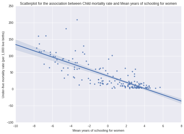
The results of the linear regression model indicates that mean years of school for women (F=245.2, p<0.0001) is significantly and negatively associated with the number of children dying under the age of five (per 1,000 live births). The F-statistic value is very high, showing that the variance between the two variables is a lot higher than the variance within each variable. The p value is considerably smaller than 0.05 which tells us that we can reject the null hypothesis of no association between child mortality rate and mean years in school for women.
Coefficient for mean years in school: Beta=-9.45, and the Intercept is 39.7.
Equation for the best fit line of the graph is: under5mort = 39.7 -9.45 * womenschool could theoretically be used to predict new values. This formula implies that increasing the average schooling of women in a country by one year, we can expect the decrease of child mortality rate by more than 9.
This is statistically significant in the model due to the F and p values previously addressed. Also given mean years in school as the only explanatory variable, this model concludes that the variability in female education level accounts for about 61.7% of the variability we have seen in child mortality rate (R2=0.617, proportion of the variance in the response variable that can be explained by the explanatory variable)
Python code
# -*- coding: utf-8 -*-
# Created on 14/08/2016
# Author Ernő Gólya

%matplotlib inline
# Import libraries
import pandas as pd
import numpy as np
import seaborn
import matplotlib.pyplot as plt
import statsmodels.formula.api as smf
#import statsmodels.stats.multicomp as multi

# Read in data file
data = pd.read_csv('custom_gapminder_2.csv', low_memory=False)

# Set variables to numeric
data["incomeperperson"] = pd.to_numeric(data["incomeperperson"],errors='coerce')
data["under5mort"] = pd.to_numeric(data["under5mort"],errors='coerce')
data["womenschool"] = pd.to_numeric(data["womenschool"],errors='coerce')
data["healthexpend"] = pd.to_numeric(data["healthexpend"],errors='coerce')

# Remove observations with NaN values in any variables of interest
# Describe function returns NaN for percentiles if dataset contains NaN
data = data.dropna()

# Create subgrup for child mortality and mean years in school
sub1 = data[['under5mort', 'womenschool']].copy()

# Center mean years in school (explanatory variable)
sub1['womenschool'] = data['womenschool'] - data['womenschool'].mean()

# Mean of womenscool
women_mean = data['womenschool'].mean()

# Print dataframe before and after centering
print "Mean of women mean years in school: %f\n" %women_mean
print "Dataframe before centering Mean years in school"
print data[['under5mort', 'womenschool']].describe(),"\n"

print "Dataframe after centering Mean years in school"
print sub1.describe()

# Regression model for schooling of women and child mortality
print "OLS regression model for the association between schooling of women and child mortality rate"
model1 = smf.ols('under5mort ~ womenschool', data=sub1).fit()
print model1.summary()

# scatterplot
fig=plt.figure(figsize=(10, 7), dpi= 80, facecolor='w', edgecolor='k')
seaborn.regplot(x='womenschool', y='under5mort', data=sub1, scatter=True)
plt.xlabel('Mean years of schooling for women')
plt.ylabel('Under-five mortality rate (per 1,000 live births)')
plt.title('Scatterplot for the association between Child mortality rate and Mean years of schooling for women');